QUESTION
This assignment will assess your fundamental understanding of aircraft performance and your
knowledge and understanding of basic Matlab coding including the use of functions, mathematical
operation and loops. You will also cover the theory of the equations covered in this assignment during
the lectures. However, they are given to you in this briefing so you can attempt the assignment before
the theory is covered in the lectures.
When you are not given the exact equations to use, you must decide what are the most appropriate
equations based on what you have learnt in the lectures – this is a key part of problem solving.
The assignment is based on the Airbus A321 for which the information you require is given in Appendix
1. In addition you will need to use air densities as given in the International Standard Atmosphere for
which values are given in Appendix 2. You should use Matlab throughout for any calculations and
plotting of results.
The assignment is divided into three parts:
1. The true airspeed of an aircraft in straight and level flight is given by
! = 2$%
&'()
where
! – true airspeed
$ – aircraft mass
% – acceleration due to gravity
& – air density
‘ – wing surface area
() – coefficient of lift
Write a function that calculates the true airspeed of the Airbus A321 where the inputs to the
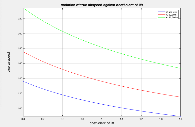
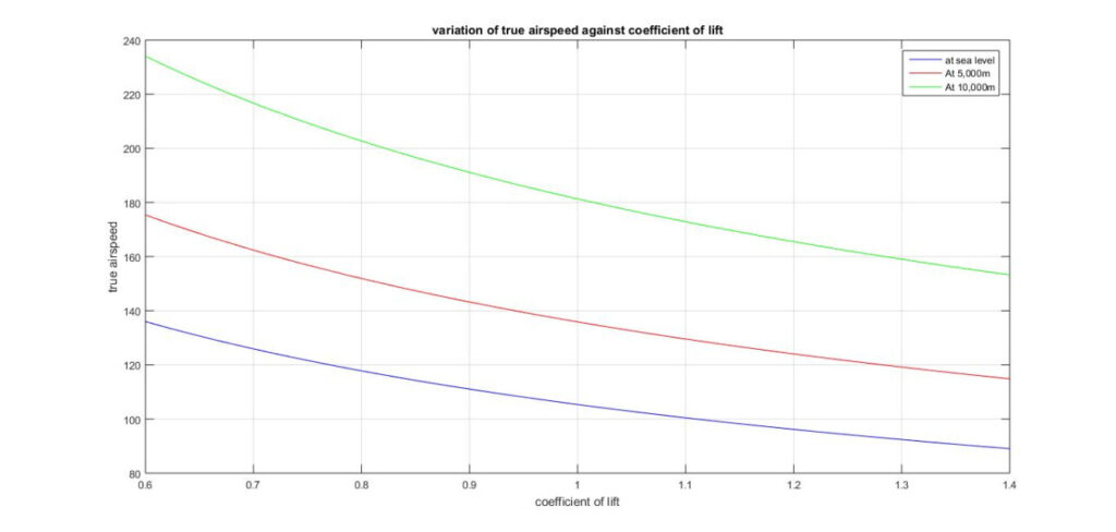
function are the aircraft mass, air density, wing surface area and CL. Using this function, write
an m-file that plots the variation in true airspeed against CL for the Airbus A321 when its mass
is 85,000kg at the altitudes of sea level, 5000m and 10,000m, i.e. you should have three
different curves on the same figure (HINT: use the command hold on to plot several lines on
the same figure). You should plot the variation for 0.6 ≤ () ≤ 1.4.
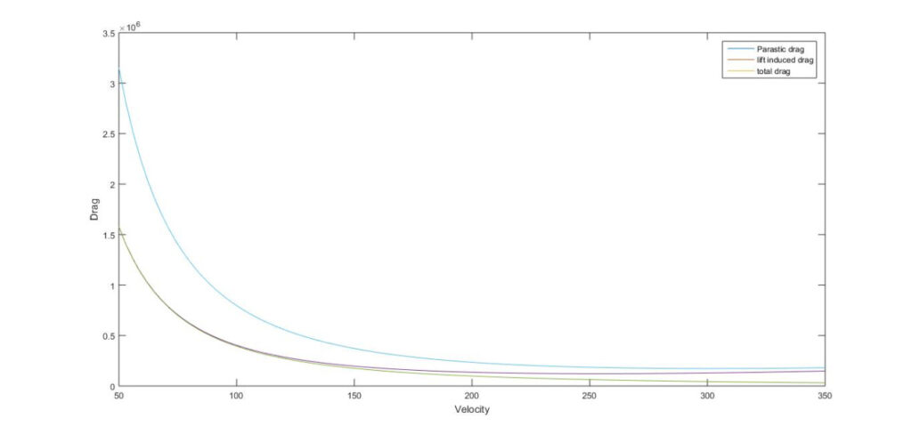
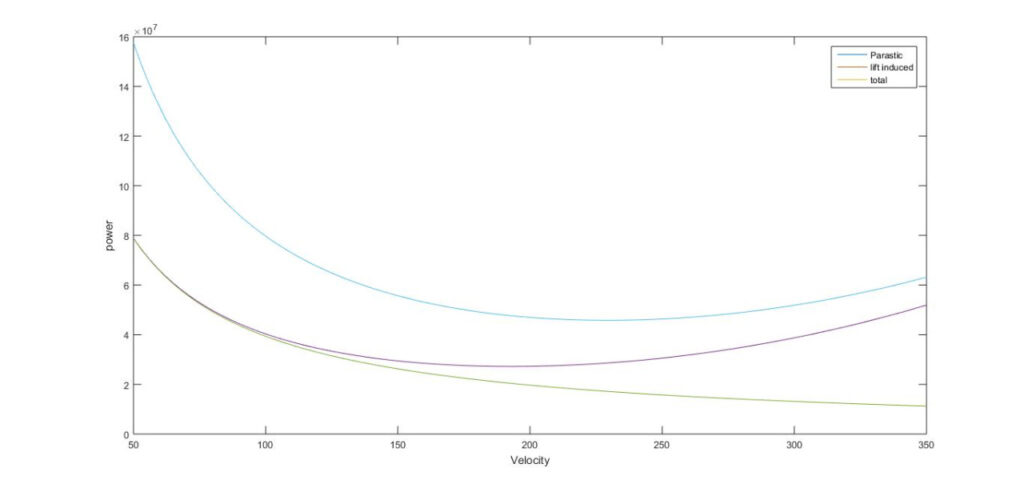
2. Write an m-file (you do not need to use functions but can if you want to) that plots the no-lift
drag and power, lift-dependent drag and power and total drag and power at the cruise altitude
against the true airspeed in the range 50m/s to 350m/s. You should use the data for the
Airbus A321 given in Appendix 1 and assume the aircraft is flying at the cruise altitude of
11,000m and that the mass is 85,000kg. You should plot the variations in drag and power
against true airspeed and you should use one figure for drag and one figure for power (you
should get graphs similar to sketches you have already seen in your lecture notes). Based on
these results what are the true airspeeds to minimise drag and power respectively?
3. During cruise, the mass of an aircraft reduces as the fuel is burnt. As a result the optimum
flight conditions will vary throughout cruise. Assuming that the Airbus A321 flies 6,100km
during this time and that the fuel burnt varies linearly with distance travelled write Matlab
code for the following.
(i) Assuming that the aircraft starts the cruise at an altitude of 10,000m and that the speed
remains constant throughout (equal to the speed calculated at the start of the cruise) plot the
variation in air density with distance travelled.
(ii) Instead, assuming that the aircraft altitude remains fixed at 10,000m, plot the variation in
speed with distance travelled.
You should assume that the Airbus A321 always flies at the minimum drag condition at
constant CL, that it starts the flight at the MTOW and flies until the MZFW.
In your answer, you need to include the equation or equations that you have used and an explanation
of how they have been used, the complete Matlab code, appropriate plots of results and a brief
discussion of the results. This assignment should take approximately 10 sides of A4 including the
Matlab code and graphs of results (this is not a page limit but a recommended length of report)
%question 1;(part1)
% ask user for values
prompt=‘please enter the aircraft mass in kg.\n’;
m=input(prompt);
prompt=‘please enter the air density in kg/m^3.\n’;
p=input(prompt);
prompt=‘please enter the wing surface area in m^2.\n’;
S=input(prompt);
prompt=‘please enter the lift coefficient.\n’;
L=input(prompt);
%intitialize value of gravitational acceleration
g=9.81;
%formula to calculate true airspeed
V=sqrt((2*m*g)/(p*S*L));
%print value to user
fprintf(‘value of the true airspeed is %d m/s’, V);
%%
% question 1; (part2)
% plot the function
% At altitude of sea level
m=85000;
p1=1.2256;
g=9.81;
S=122.6;
V1=@(L) sqrt((2.*m.*g)./(p1.*S.*L));
%At altitude of 5,000 m
p2=0.7368;
V2=@(L) sqrt((2.*m.*g)./(p2.*S.*L));
% At altitude of 10,000 m
p3=0.4138;
V3=@(L) sqrt((2.*m.*g)./(p3.*S.*L));
fplot(V1,[0.6 1.4], ‘b’);
hold on
fplot(V2,[0.6 1.4],‘r’);
hold on
fplot(V3,[0.6 1.4],‘g’);
grid on
title(‘variation of true airspeed against coefficient of lift’);
xlabel(‘coefficient of lift’);
ylabel(‘true airspeed’);
legend(‘at sea level’, ‘At 5,000m’, ‘At 10,000m’);
% Plot of variation of true airspeed against coefficient of lift
%%
% question2;(part1)
% Finding the coefficient of lift in order to calculate the coefficient of
% darg,
% Where l=w=mg=(85,000)*(9.81)=833850 N ,at level of flight ,
% At altitude of 11,000m
l=833850;
S=122.6;
g=9.81;
x=6100;
m=85000;
p=0.3650;
V=[50 350];
CL=(2.*l)./(p.*(V.^2)*S);
%To find CD,
%Where’s R=0.0424 ,U=0.1267
CD=0.0424+0.1267.*(CL^2);
%Then value of of CD is ,,,
% To find no-lift dependent drag (parasite drag),
Dp=((0.5).*p.*(V.^2).*S.*CD);
Di=(U.*(m.*g)^2/(0.5).*p.*(V.^2)*S);
%Then to find the total darg (Dt),
Dt=Dp+Di;
%PLOT THE FUNCTION,
%plot drag against the true airspeed,
fplot(Dp,V);
hold on
fplot(Di,V);
hold on
fplot(D,V);
% To find power p1 (for the parasite darg),
p1=Dp*V;
% TO find power p2(for the induced drag),
p2=Di*V;
% In order to work out the power(po),
po=Dt.*V;
%plot power against the the true airspeed;
plot(p1,V);
hold on
plot(p2,V);
hold on
plot(po,V);
QUESTION3 ON THE BOTTOM LAST PAGE
%%
% question3;
%first part of the question ,
% At altitude of 10,000m
% To find the coefficient of lift ,
CDo=0.0424;
e=0.1267;
CL=sqrt((CDo)./e)
%Therefore the value of CL=0.5785,
% Finding the true airspeed;
m=85000;
g=9.81;
S=122.6;
p=0.4138;
v=sqrt((2.*m.*g)./(p.*S.*CL))
%Therefore the value of v=238.3807,
%% In order to find change in mass ,[AS the fuel burnt varies linearly with distance travelled]
% (0,85000) (6100,73800)
% Gradient=-1.836065574 that is fuel consumption per meter ,
% USING THE EQUATION OF STRIGHT LINE Y-Yo=M(X-Xo) Gives the following ,,
% y-85000=-1.836065574(X-0)
%y=mass(M) =-1.836065574x+8500
% By subs m into v-Equation,
% In-order to plot the variation of air density against distance travelled,
% At altitude 10,000m,
X=[0 6100];
v=238.3807
M=-1.836065574.*X.+85000;
S=122.6;
CL= 0.5785;
g=9.81;
p=@(X) (2.*g.*(-1.836065574.*X.+85000)./(v^2.*S.*CL)
fplot(p,[0 6100],‘r’);
(DON’T LOOK TO THIS PART ) QUESTION 3 ON THE BOTTOM OF THE PAGE >>
%%
% question3;
%first part of the question ,
% At altitude of 10,000m
% To find the coefficient of lift ,
% Where l=w=mg=(85,000)*(9.81)=833850 N ,at level of flight ,
l=833850;
S=122.6;
g=9.81;
x=6100;
m=85000;
p=0.4138;
V=[50 350];
CL=@(V) (2*l)/(p*V^2*S)
% In order to find change in mass ,[AS the fuel burnt varies linearly with distance travelled]
% (0,85000) (6100,73800)
% Gradient(M)=-1.836065574 that is specific fuel consumption ,
% USING THE EQUATION OF STRIGHT LINE Y-Yo=M(X-Xo) Gives the following ,,
% y-85000=833850(X-0)
%y=mass(m)=833850x+85000
% By subs M into v-Equation,
X=[0 6100];
M=833850*X+85000;
v=@(P) sqrt((2.*M.*g)./(P.*S.*CL));
%% In-order to plot the variation of air density against distance travelled,
% At altitude 10,000m,
p=0.4138;
x=6100;
M=833850*X+85000;
S=122.6;
CL=@(V) (2*l)/(p*V^2*S);
g=9.81;
v=sqrt((2.*M.*g)./(p.*S.*CL));
%Plot the variation of true airspeed against
X=[0,6100];
S=122.6;
g=9.81;
CL=0.5785;
V=sqrt((2.*M.*g)./(p.*S.*CL))
ANSWER
%question 1;(part1)
% ask user for values
prompt=’please enter the aircraft mass in kg.\n’;
m=input(prompt);
prompt=’please enter the air density in kg/m^3.\n’;
p=input(prompt);
prompt=’please enter the wing surface area in m^2.\n’;
S=input(prompt);
prompt=’please enter the lift coefficient.\n’;
L=input(prompt);
%intitialize value of gravitational acceleration
g=9.81;
%formula to calculate true airspeed
V=sqrt((2*m*g)/(p*S*L));
%print value to user
fprintf(‘value of the true airspeed is %d m/s’, V);
%%
% question 1; (part2)
% plot the function
% At altitude of sea level
m=85000;
p1=1.2256;
g=9.81;
S=122.6;
V1=@(L) sqrt((2.*m.*g)./(p1.*S.*L));
%At altitude of 5,000 m
p2=0.7368;
V2=@(L) sqrt((2.*m.*g)./(p2.*S.*L));
% At altitude of 10,000 m
p3=0.4138;
V3=@(L) sqrt((2.*m.*g)./(p3.*S.*L));
fplot(V1,[0.6 1.4], ‘b’);
hold on
fplot(V2,[0.6 1.4],’r’);
hold on
fplot(V3,[0.6 1.4],’g’);
grid on
title(‘variation of true airspeed against coefficient of lift’);
xlabel(‘coefficient of lift’);
ylabel(‘true airspeed’);
legend(‘at sea level’, ‘At 5,000m’, ‘At 10,000m’);
% Plot of variation of true airspeed against coefficient of lift
% question2;(part1)
% Finding the coefficient of lift in order to calculate the coefficient of
% darg,
% Where l=w=mg=(85,000)*(9.81)=833850 N ,at level of flight ,
% At altitude of 11,000m
l=833850;
S=122.6;
g=9.81;
x=6100;
m=85000;
p=0.3650;
V=linspace(50,350);
CL=(2*m*g)./(p*(V.^2)*S);
%To find CD,
%Where’s R=0.0424 ,U=0.1267
U=0.1267;
CD=0.0424+0.1267*(CL.^2);
%Then value of of CD is ,,,
% To find no-lift dependent drag (parasite drag),
for i=1:100
Dp(i)=((0.5)*p*(V(i).^2)*S*CD(i));
Di(i)=((U*(m*g)^2)/((0.5)*p*(V(i).^2)*S));
%Then to find the total darg (Dt),
Dt=Dp+Di;
end
%PLOT THE FUNCTION,
%plot drag against the true airspeed,
figure(1)
plot(V,Dp);
hold on
plot(V,Di);
hold on
plot(V,Dt);
hold on
legend(‘Dp’, ‘Di’, ‘Dt’);
% To find power p1 (for the parasite darg),
p1=Dp.*V;
% TO find power p2(for the induced drag),
p2=Di.*V;
% In order to work out the power(po),
po=Dt.*V;
%plot power against the the true airspeed;
figure(2)
plot(p1,V);
hold on
plot(p2,V);
hold on
plot(po,V);
%% question3;
%first part of the question ,
% At altitude of 10,000m
% To find the coefficient of lift ,
% Where l=w=mg=(85,000)*(9.81)=833850 N ,at level of flight ,
l=833850;
S=122.6;
g=9.81;
x=6100;
m=85000;
p=0.4138;
V=[50 350];
CL=@(V) (2*l)/(p*V^2*S)
% In order to find change in mass ,[AS the fuel burnt varies linearly with distance travelled]
% (0,85000) (6100,73800)
% Gradient(M)=-1.836065574 that is specific fuel consumption ,
% USING THE EQUATION OF STRIGHT LINE Y-Yo=M(X-Xo) Gives the following ,,
% y-85000=833850(X-0)
%y=mass(m)=833850x+85000
% By subs M into v-Equation,
X=[0 6100];
M=833850*X+85000;
v=@(P) sqrt((2.*M.*g)./(P.*S.*CL));
%% In-order to plot the variation of air density against distance travelled,
% At altitude 10,000m,
p=0.4138;
X=6100;
M=833850*X+85000;
S=122.6;
CL=@(V) (2*l)/(p*V^2*S);
g=9.81;
v=sqrt((2.*M.*g)./(p.*S.*CL));
%Plot the variation of true airspeed against
X=[0,6100];
S=122.6;
g=9.81;
CL=0.5785;
V=sqrt((2.*M.*g)./(p.*S.*CL))
PLOT
Looking for best MATLAB Assignment Help. Whatsapp us at +16469488918 or chat with our chat representative showing on lower right corner or order from here. You can also take help from our Live Assignment helper for any exam or live assignment related assistance.