Confidence Interval for Percentage-Statistics Assignment Sample

QUESTION

 

Problem 1

The data set “STAT 250 Final Exam Scores” contains a random sample of 269 STAT 250 students’ final exam scores (maximum of 80) collected over the past two years. Answer the following questions using this data set.

STAT 250 Final Exam Scores

Scores
29
30
31
32
33
34
34
34
35
35
35
36
36
36
36
37
37
37
38
39
39
39
40
40
40
41
42
42
42
42
42
42
42
42
42
43
43
43
44
44
44
44
44
45
45
45
45
46
46
46
47
47
47
47
47
47
47
47
47
47
47
48
48
48
48
48
48
48
48
48
48
49
49
49
49
50
50
50
50
50
50
50
50
50
50
50
50
51
52
52
52
52
52
52
52
52
52
52
52
52
53
53
53
53
54
54
54
54
54
54
54
54
54
54
54
55
55
55
55
55
55
55
55
56
56
56
56
56
56
56
56
56
56
56
57
57
57
57
57
57
57
57
57
57
57
57
57
58
58
58
58
58
58
58
59
59
59
59
59
59
60
60
60
60
60
60
60
61
61
61
61
61
61
61
62
62
62
62
62
62
62
62
62
63
63
63
63
63
63
63
63
63
63
64
64
64
64
64
64
64
65
65
65
65
65
65
65
65
65
65
65
66
66
66
66
66
66
66
66
66
66
66
66
67
67
68
68
68
68
68
69
69
69
70
70
70
70
70
71
71
71
71
71
71
72
72
72
72
72
72
73
73
74
74
74
75
75
75
76
76
76
76
76
77
78
78
79
80
80

  a. What proportion of students in our sample earned A’s on the final exam? A letter grade of A is obtained with a score of 72 or higher. Hint: You can do this many ways, but in StatCrunch, go to Data  Row Selection  Interactive Tools. In the slider selectors box, click the variable “Scores” into the variable box. Then click compute. Use the slider to obtain the count by looking at the “# rows selected” presented in the first line of the box. Show your work (i.e. describe the method you used to obtain the number of A’s) and express this value as a proportion rounded to four decimal places.

2. Assuming there is a big population of students who have completed the final exam in STAT 250, write one sentence each to check the two other conditions of the Central Limit Theorem.

3. Using the sample proportion obtained in (a), construct a 95% confidence interval to estimate the population proportion of students who earned an A on the final exam. Please do this “by hand” using the formula and showing your work (please type your work, no images accepted here). Round your confidence limits to four decimal places.

4. Verify your result from part (b) using Stat  Proportions Stats  One Sample  With Summary. Inside the box, enter the number of students who earned an A as the # of successes, the sample size as the # of observations, and select confidence interval and click Compute! Copy and paste your StatCrunch result in your document.
5. Interpret the StatCrunch confidence interval in part (c) in one sentence using the context of the question.

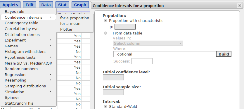
6. Use the Confidence Interval applet (for a Proportion) in StatCrunch to simulate constructing one thousand 95% confidence intervals assuming the proportion of A’s in the population is p = 0.11 and the sample size n = 269. Once the window is open, click reset and select (or click) 1000 intervals. Copy and paste your image into your document.

7. Compare the “Prop. contained” value from part (f) to the confidence level associated with the simulation in one sentence.
8. Write a long-run interpretation for your confidence interval method in context in one sentence.

Problem 2: Food Delivery Robots

As we all know, GMU began a robot food delivery service in January. One of the potential benefits of this service is to help the busiest students eat breakfast. Research has shown that about 88% of college students skip breakfast due to busy schedules and other reasons. Initial data were collected from a random sample of 291 Mason students who utilize the robot food delivery service and are presented in StatCrunch. The responses (0 = ate breakfast and 1 = did not eat breakfast) are found in StatCrunch in a data set called “Food Delivery Robots.”

1. 1. 1. 1. Obtain the sample proportion of individuals who said “they did not eat breakfast” using Stat  Tables  Frequency in StatCrunch. Only the value of the sample proportion is needed in your answer. Present this sample proportion as a decimal rounded to 4 decimal places.

1. 1. 1. 2. Using  = 0.05, is there sufficient evidence to conclude that less than 88% GMU students who utilize the food delivery robots skip breakfast? Conduct a full hypothesis test by following the steps below.

1. Define the population parameter in one sentence.
2. State the null and alternative hypotheses using correct notation.
3. State the significance level for this problem.
4. Check the three conditions of the Central Limit Theorem that allow you to use the one-proportion z-test using one complete sentence for each condition. Show work for the numerical calculation. Assume the population is large.
5. Calculate the test statistic “by-hand.” Show the work necessary to obtain the value by typing your work and provide the resulting test statistic. Do not round while doing the calculation. Then, round the test statistic to two decimal places after you complete the calculation.
6. Calculate the p-value using the standard Normal table and provide the answer. Use four decimal places for the p-value.
7. State whether you reject or do not reject the null hypothesis and the reason for your decision in one sentence (compare your p-value to the significance level to do this).
8. State your conclusion in context of the problem (i.e. interpret your results and/or answer the question being posed) in one or two complete sentences.
9. Use StatCrunch (Stat  Proportion Stats  One Sample  with Data) to verify your test statistic and p-value. Copy and paste this box into your document.

Problem 3: Shuttle Service

Officials are trying to determine if they are using the correct number of campus shuttles for the number of individuals who use them. If the proportion of individuals associated with (including faculty, staff, and students) who use the shuttles is significantly different from 0.28, the officials believe they will have to either remove or add a shuttle to the fleet. In a random sample of 444 people taken from the population of all individuals associated with (including faculty, staff, and students) it was discovered that 123 of these individuals use the shuttle.

1. Check the three conditions of the Central Limit Theorem that allow you to use the one-proportion confidence interval using one complete sentence for each condition. Show work for the numerical calculation.

2. Construct a 99% confidence interval to estimate the population proportion of these individuals who use the shuttle system. Calculate this “by hand” using the formula and showing your work (please type your work, no images accepted here). Round your confidence limits to four decimals.

3. Verify your result in part (b) using Stat  Proportions Stats  One Sample  With Summary. Copy and paste your StatCrunch result in your document as well.

4. Using  = 0.01, is there sufficient evidence to conclude that the proportion of the individuals who use shuttles is different from 0.28? Conduct a full hypothesis test by following the steps below. Enter an answer for each of these steps in your document.

1. Define the population parameter in one sentence.
2. State the null and alternative hypotheses using correct notation.
3. State the significance level for this problem.
4. Calculate the test statistic “by-hand.” Show the work necessary to obtain the value by typing your work and provide the resulting test statistic. Do not round during the calculation. Then, round the test statistic to two decimal places after you complete the calculation.
5. Calculate the p-value using the standard Normal table and provide the answer. Use four decimal places for the p-value.
6. State whether you reject or do not reject the null hypothesis and the reason for your decision in one sentence (compare your p-value to the significance level to do this).
7. State your conclusion in context of the problem (i.e. interpret your results and/or answer the question being posed) in one or two complete sentences.
8. Use StatCrunch (Stat  Proportion Stats  One Sample  with Summary) to verify your test statistic and p-value. Copy and paste this box into your document.

5. Explain the connection between the confidence interval and the hypothesis test in this problem (discuss this in relation to the decision made from your hypothesis test and connect it to the confidence interval you constructed in part (b)). Answer this question in one to two sentences.

Problem 4: Building another Sampling Distribution

We will use the Sampling Distribution applet in StatCrunch to investigate properties of sampling distributions of the mean for a right skewed distribution. Under Applets, open the Sampling distribution applet (box shown below). First, select “right skewed” for the population and then click on Compute.

1. Once the applet box is opened, enter 5 in the box to the right of the words “sample size” in the right middle of the applet box window. Then, at the top of the applet, click “1 time.” Watch the resulting animation. When the sample is completed, copy and paste the entire applet box (using options  copy) into your document.

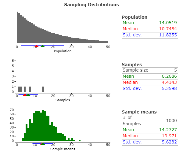
3. Click Reset at the top of the applet. Then, click the “1000 times” to take 1000 samples of size 5. Copy and paste the applet image into your document.
4. Describe the shape of the Sample means graph at the bottom of your image from part (b) in one sentence.
5. Why do you think that this graph does not have an approximately Normal shape? Use the Central Limit Theorem large sample size condition (for means) to answer this question in one sentence.
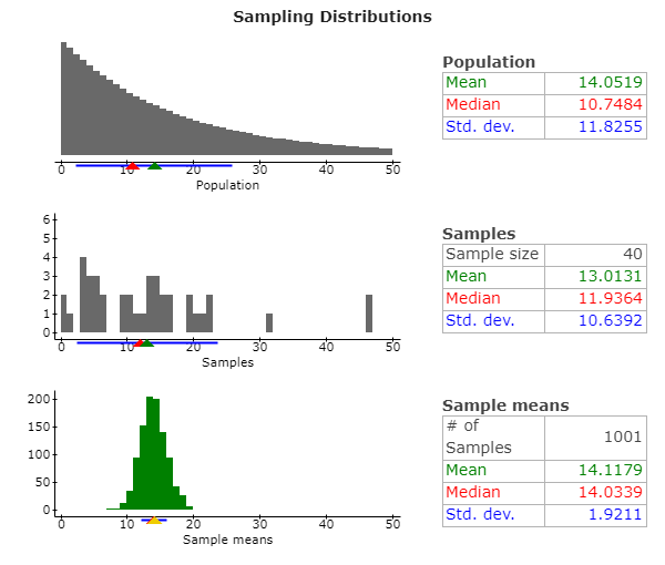
6. Click Reset at the top of the applet. Type 40 in the sample size box. Then, click the “1000 times” to take 1000 samples of size 40. Copy and paste the applet image into your document.
7. Describe the shape of the Sample Proportions graph at the bottom of your image from part (e) in one sentence.
8. Why do you think that this graph from part (f) has the shape you described? Use the Central Limit Theorem large sample size condition to answer this question in one sentence.
9. Using the image in part (e), write the values you obtained for the mean (in green) and the standard deviation (in blue). These values are found in the bottom right box labeled “Sample Means”
10. Compare the mean value (in green, found in part (h)) to the known mean of the population from the top box labeled “Population.”
11. Now calculate the standard error of the sample mean using the value labeled “Std. dev.” in blue from the top box. Round this value to three decimal places.
12. Compare the value in part (j) to the standard deviation (in blue) you obtained in part (h) in one sentence.
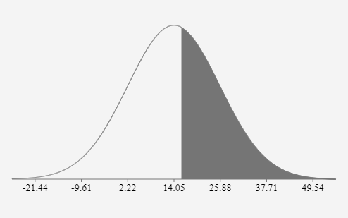
13. Assuming this right skewed population distribution had a population mean of 14.05 and a standard deviation of 11.83; calculate the probability that, in a random sample of 30, the mean of the sample is greater than 16. First, draw a picture with the mean labeled, shade the area representing the desired probability, standardize, and use the Standard Normal Table (Table 2 in your text) to obtain this probability. Please take a picture of your hand drawn sketch and upload it to your Word document (if you do not have this technology, you may use any other method (i.e. Microsoft paint) to sketch the image). You must type the rest of your “by hand” work to earn full credit.
14. Verify your answer in part (l) using the StatCrunch Normal calculator and copy that image into your document. In addition, write one sentence to explain what the probability means in context of the question.

 

ANSWER

 

Problem 1

(a) Sol. We selected all the values in the range of 72-80. Total no of values with A grade = 25.

Total no of students = 269.

Req. no of proportions = 25/269 = 0.0929

(b) Sol. If there is a big population of students who have completed their final exam, then the two conditions to check for Central Limit Theorem are Randomization Condition and Sample Size Assumption. The data has been randomly sampled in this case. The sample size is 269, which is sufficiently large.

(c) Sol. For 95% CI, z value = 1.96.

Proportion of positive result = 0.0929

SEM = (0.0929*0.9071/269)^0.5 = 0.0177

Lower Bound = 0.0929 – 1.96*SEM = 0.0929 – 0.0347 = 0.1276

Upper Bound = 0.0929 + 1.96*SEM = 0.0929 + 0.0347 = 0.0582

(d) Sol. Output is as below: –

One sample proportion summary confidence interval:

p : Proportion of successes
Method: Standard-Wald

95% confidence interval results:

Proportion	Count	Total	Sample Prop.	Std. Err.	L. Limit	U. Limit
p	25	269	0.092936803	0.017702577	0.058240389	0.12763322

(e) Sol. With 95% confidence, we can say that the proportion of students lies in the range of 0.1276 to 0.0582.

(f) Sol.

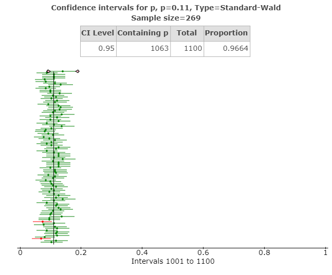
(g) Sol. Proportion contained in the case is 0.9664 as can be seen from the above figure. The no of values containing p is 1063.

(h) Sol. The long run interpretation for the confidence interval has been shown in the above figure. A large proportion of the sample means lie on the right-hand side of the given success value of 0.11. Only two runs (in red) can be seen as completely shifted over left hand side of the given success value.

 

Problem 2

(a) Sol.

Frequency table results for Breakfast?: 

Count = 291

Breakfast?	Frequency	Relative Frequency
0	47	0.16151203
1	244	0.83848797

 

(b) Sol.

1. College students form the population parameter in this hypothesis test. The sample consists of 291 GMU college students.
2. H₀: The proportion of students who utilize the food delivery robots and skip their breakfast is greater than or equal to 0.88.

H_A: The proportion of students who utilize the food delivery robots and skip their breakfast is less than 0.88.

3. Significance level for this problem is 0.05.
4. p = 244/291 = 0.8385, (1-p) = 0.1615, n = 291

np = 291*0.8385 = 244.0035, n(1-p) = 291*0.1615 = 46.9965

Both the values are greater than 5, which satisfies the dichotomous outcome for the Central Limit theorem.

The sample has been chosen as a random sample, and hence, it satisfies the independent sampling and randomization sampling condition.

The sample size in this problem is 291, and it is sufficiently large. According to the Central Limit Theorem, for illustrating a normal distributed characteristic, the sample size should be greater than 30.

5. Test statistic = (0.8385 – 0.88)/[0.88*(1-0.88)/291]^0.5 = – 2.18
6. For the given statistic, p-value = 0.0147
7. As p-value is lesser than 0.05, we reject the null hypothesis.
8. Hence, we can say that the proportion of students who utilize the food delivery robots and skip their breakfast is less than 0.88.
9. Below is the output

One sample proportion summary hypothesis test:

p : Proportion of successes
H₀ : p = 0.88
H_A : p < 0.88

Hypothesis test results:

Proportion	Count	Total	Sample Prop.	Std. Err.	Z-Stat	P-value
p	244	291	0.83848797	0.019049583	-2.1791568	0.0147

 

Problem 3

(a) Sol. Total sample size = 444

No of people using shuttle service = 123

p = 123/444 = 0.277, (1-p) = 0.723

The sample size is 444, which is greater than the acceptable limit of 30 for illustrating a normal distribution characteristic.

Both np and n(1-p) are greater than 5, which shows the possibility of dichotomous variable being successful in this case.

The sample has been taken randomly from the campus, and it is independent of other samples. So, it satisfies the Randomization condition for the Central Limit Theorem.

(b) Sol. For a 99% CI, Z score for a two tailed test = 2.576

Standard Error of Mean = 0.0212

Lower Bound = p – (Z*SEM) = 0.277 – (2.576*0.0212) = 0.277 – 0.0547 = 0.2223

Upper Bound = p + (Z*SEM) = 0.277 + (2.576*0.0212) = 0.277 + 0.0547 = 0.3317

(c) Sol. Below is the output

One sample proportion summary confidence interval:

p : Proportion of successes
Method: Standard-Wald

99% confidence interval results:

Proportion	Count	Total	Sample Prop.	Std. Err.	L. Limit	U. Limit
p	123	444	0.27702703	0.021238831	0.22231942	0.33173463

(d) Sol. Office going individuals are the population parameter in this case.

H₀: The proportion of office going individuals who use the shuttle service is equal to 0.28.

H_A: The proportion of office going individuals who use the shuttle service is not equal to 0.28.

Significance level for this problem is 0.01.

Test statistic = (0.277 – 0.28)/(0.28*0.72/444)^0.5 = – 0.14

Z_critical = 2.58

For this test statistic, p value = 0.889

As p-value is greater than our acceptable significance level, we fail to reject the null hypothesis. We don’t have enough evidence to reject the null hypothesis.

Hence, we can say that the proportion of office going individuals who use the shuttle service is equal to 0.28.

One sample proportion summary hypothesis test:

p : Proportion of successes
H₀ : p = 0.28
H_A : p ≠ 0.28

Hypothesis test results:

Proportion	Count	Total	Sample Prop.	Std. Err.	Z-Stat	P-value
p	123	444	0.27702703	0.021308544	-0.13952023	0.889

(e) Sol. The confidence interval that we conducted in this case ranges from 0.2223 to 0.3317. The hypothesis test has been made with the proportion being equal to 0.28. So, it lies almost in between the confidence interval range. Hence, we don’t have enough evidence to reject the null hypothesis.

 

Problem 4

(a) Sol.

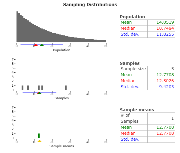
(b) Sol.

(c) Sol. It can be observed that the sample means graph in the previous part is illustrating similar to the shape of a slight right skewed distribution.

(d) Sol. The graph doesn’t resemble that of a normal distribution. According to the Central Limit Theorem, the distribution of a sample means resemble the normal distribution only when the sample sizes are greater than 30. In this case, the sample size is 5, which is why it doesn’t meet the condition.

(e) Sol.

(f) Sol. The shape of the sample means distribution resembles to that of a normal distribution.

(g) Sol. The shape of the above distribution being similar to normal distribution is due to the sample size of the samples being equal to 40, which is greater than the acceptable sample size of 30 for being the normal distribution sample, according to the Central Limit Theorem.

(h) Sol. The mean of the sample means comes out to be 14.1179, whereas the standard deviation of the sample means comes out to be 1.9211.

(i) Sol. The mean of the sample means (14.1179) is higher than the mean of the population (14.0519), however the difference not being a majorly significant one.

(j) Sol. Standard error of the mean = 11.8255/(40)^0.5 = 1.87

(k) Sol. The standard error of the mean is 1.87, which is almost equal to the standard deviation of the sample means (1.9211).

(l) Sol.

Probability for the mean of sample being greater than 16 = 0.4345

(m) Sol. The output is as follows: –

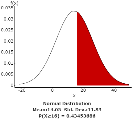
It means that there is 43.45% probability that the value of the mean of any random sample taken is greater than 16.