QUESTION
PART ONE
A researcher is interested in quantifying the relationship between the salary of a Board Member in a
company and other factors such as the size of the Board (including Executives and Nonexecutives), the
number of committees that the Board members are involved, Type of industry, and the level of success of
the company. To this end, he has compiled an Excel file (Data 2A_Assignment 2_S3 2019 LSBF.xls) that
contains 75 members of boards from public companies listed on ASX. The variables included are as follows:
SALARY Salary in $A
EXECUTIVES Number of EXECUTIVE board members
NONEXECUTIVES Number of NONEXECUTIVE board members
COMMITTEE Number of COMMITTEEs that board member is involved
TYPE TYPE of industry (1= Mining, 2 = Energy 3 = Financial Services, 4 =
Manufacturing, 5 = Utilities)
SUCCESS Level of SUCCESS (1= the worst, 5=the best)
Note that TYPE and SUCCESS are two categorical variables and four dummy variables for each of these
categorical variables are included in the data file. TYPE 1 and SUCCESS 1 are considered as the base level.
Use SPSS to conduct the regression analysis and inform the agent with regards to the results of the analysis. In
interpreting the SPSS results, you may have to answer the following questions.
(1) Using Ordinary Least Square (OLS) method estimate the regression model. The below is the
estimating model to help with model estimation (hint: use the estimated coefficients to write the regression
equation using the following model).
SALARY = β0 + β1 EXECUTIVES + β2 NONEXECUTIVES + β3 COMMITTES + β4 T2 +
β5 T3 + β6 T4 + β7 T5 + β8 S2 + β9 S3 + β10 S4 + β11 S5 + ε
(2) What are the a priori signs of the coefficients based on your experience or theories and are they the
same as the signs of the estimated coefficients from the model in the SPSS output? If you find that
the signs are not as you expected, you may need further explanations as to why this is the case.
(3) Interpret the meanings of slopes of this model and check whether these coefficients are significant.
(4) Use the adjusted R2 and CV to evaluate the goodness of fit of the model.
(5) Using ANOVA statistics check also whether the model is significant.
(6) Is there any evidence that the regression might have problems associated with multi-collinearity, heteroskedasticity or non-normality of the regression residuals?
(7) Using the regression model estimated, predict the SALARY of a board member in a company with 4
Executives, 2 Nonexecutives, 5 Committees, Industry Type of 3, and a Success level of 4.
PART TWO
A large number of decisions involved in the consumer lending business require the application of models
that are based on personal characteristics including marital status, age, income and other factors. The file
Data 2B_Assignment2_S3 2019 LSBF.xls has been compiled with 150 observations from a random
sample of borrowers who are in full-time or part-time employment.
The bank of Victoria’s lending manager wants to develop a credit risk model that distinguishes between
populations of good and bad borrowers. The good borrower pays principal and interest on time. The bad
borrower may default a part or the full payment of principal and interest. The survey that is used to compile
the data file dealt with whether respondents are good or bad borrowers and their attitudes towards the bank
loan. The following variables are included:
Borrower 1 if the borrower is a good borrower, 0 otherwise
Age age in years
Income borrower’s annual earnings in $K
Marital 1 if the person is married, 0 otherwise
Profession 1 if the borrower is in full-time employment, 0 otherwise
Gender 1 = male, 0 = female
Borrowers are also asked their responses to six statements concerning the loan. The statements and the
variable names are:
Cheaper “It is cheaper to borrow from the bank of Victoria than to borrow from the other
banks.”
Mode “I am willing to apply for online borrowing mode if available.”
Useful “Online applications are useful to people who surf the Internet frequently.”
Informative “I gain a lot of information from reading the PDS (Product Disclosure Statement)
of the loan.”
Payment “I borrow from the bank that charges application fee of not more than $100.”
Current “Consumer loan supports my daily life.”
The responses to the attitudinal questions are coded as follows:
1 = strongly disagree
2 = disagree
3 = no view either way
4 = agree
5 = strongly agree
Use SPSS to perform a discriminant analysis in which the dependent variable is BORROWER and the
independent variables are AGE, INCOME, MARITAL, PROFESSION, and GENDER.
(8) Hold out the last 50 observations from the analysis.
(9) Generate means, univariate ANOVAs, unstandardised function coefficients, within-groups
correlations and a summary table.
(10) Estimate the discriminant function and analyse all tables in your report.
(11) Using the discriminant function estimated in your analysis, determine whether the person with the
following characteristics is likely to be a good borrower or otherwise:
A 45 years old married male in part-time employment and earns an annual income of $55,000.
PART THREE
Use SPSS to perform a factor analysis of the six attitudinal variables and analyse all tables in your report.
(12) Produce univariate descriptive statistics and correlation coefficients. Use principal components to
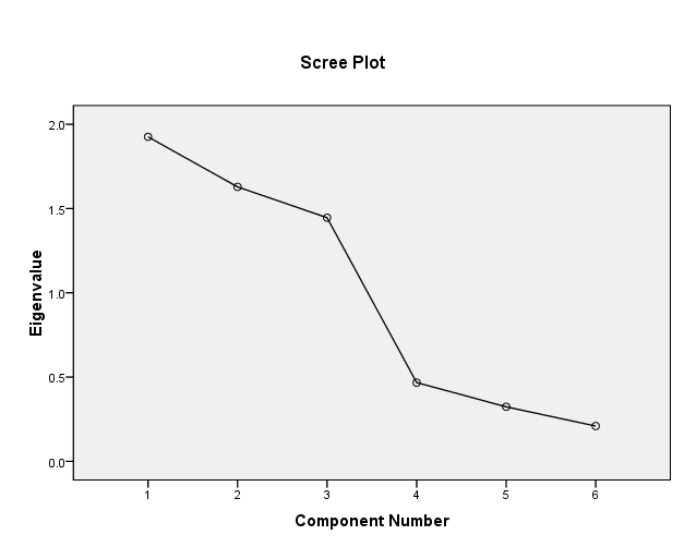
extract the factors and varimax to rotate the factors. Also produce a scree plot and identify the factors.
(13) Save the factors and use them in a discriminant analysis together with the independent variables
AGE, INCOME, MARITAL, PROFESSION, and GENDER.
(14) Does using the factors improve the discriminant analysis?, Explain why?
Presentation: General guidelines
1. Your assignment must be presented on Microsoft Word. Copy and paste all SPSS output to this
MS Word document. Make sure the document is a single sided print.
2. You are required to write the report to suit the academic standards.
3. Attach an assignment declaration with your name and ID numbers clearly written.
4. All tables and figures should contain a title that clearly explains the content.
5. SPSS tables, once copied to word file should be formatted to suite the presentation of report.
6. Interpretations should be precise and you are required to use the plain language
7. Assignments without interpretations will attract low marks.
8. An electronic copy of the assignment should be submitted to the drop box in VUC Space of the
unit.
9. Download the similarity report and attach the report to the hard copy of your assignment.
10. Submit the hard copy of the assignment personally to your tutor for marking. This must be securely
stapled in the top left hand corner.
(Data 2A_Assignment 2_S3 2019 LSBF.xls)(Excel File)
| Salary | EXECUTIVES | NONEXECUTIVES | COMMITTEE | T2 | T3 | T4 | T5 | S2 | S3 | S4 | S5 |
| 367000 | 2 | 1 | 2 | 1 | 0 | 0 | 0 | 1 | 0 | 0 | 0 |
| 368000 | 3 | 1 | 3 | 1 | 0 | 0 | 0 | 1 | 0 | 0 | 0 |
| 368000 | 3 | 1 | 3 | 1 | 0 | 0 | 0 | 1 | 0 | 0 | 0 |
| 369000 | 2 | 1 | 3 | 1 | 0 | 0 | 0 | 0 | 1 | 0 | 0 |
| 372000 | 4 | 2 | 5 | 1 | 0 | 0 | 0 | 1 | 0 | 0 | 0 |
| 375000 | 2 | 1 | 3 | 0 | 1 | 0 | 0 | 0 | 0 | 1 | 0 |
| 376000 | 2 | 1 | 2 | 1 | 0 | 0 | 0 | 0 | 1 | 0 | 0 |
| 376900 | 3 | 1 | 3 | 1 | 0 | 0 | 0 | 0 | 1 | 0 | 0 |
| 377000 | 2 | 3 | 5 | 1 | 0 | 0 | 0 | 0 | 1 | 0 | 0 |
| 378000 | 2 | 1 | 2 | 0 | 1 | 0 | 0 | 1 | 0 | 0 | 0 |
| 379000 | 3 | 2 | 3 | 1 | 0 | 0 | 0 | 0 | 1 | 0 | 0 |
| 380000 | 3 | 1 | 2 | 1 | 0 | 0 | 0 | 0 | 1 | 0 | 0 |
| 380000 | 3 | 1 | 2 | 1 | 0 | 0 | 0 | 0 | 1 | 0 | 0 |
| 381000 | 2 | 1 | 3 | 0 | 1 | 0 | 0 | 0 | 1 | 0 | 0 |
| 382000 | 3 | 1 | 3 | 1 | 0 | 0 | 0 | 0 | 1 | 0 | 0 |
| 383000 | 3 | 1 | 3 | 1 | 0 | 0 | 0 | 0 | 1 | 0 | 0 |
| 384000 | 3 | 1 | 3 | 1 | 0 | 0 | 0 | 1 | 0 | 0 | 0 |
| 384000 | 3 | 1 | 3 | 1 | 0 | 0 | 0 | 0 | 1 | 0 | 0 |
| 386250 | 4 | 2 | 3 | 0 | 0 | 0 | 0 | 0 | 0 | 1 | 0 |
| 387000 | 3 | 2 | 2 | 0 | 1 | 0 | 0 | 0 | 1 | 0 | 0 |
| 389500 | 3 | 2 | 2 | 0 | 1 | 0 | 0 | 1 | 0 | 0 | 0 |
| 390400 | 4 | 2 | 4 | 1 | 0 | 0 | 0 | 0 | 0 | 1 | 0 |
| 390500 | 3 | 1 | 3 | 0 | 1 | 0 | 0 | 0 | 1 | 0 | 0 |
| 391000 | 3 | 2 | 3 | 0 | 1 | 0 | 0 | 0 | 1 | 0 | 0 |
| 391500 | 4 | 2 | 3 | 0 | 1 | 0 | 0 | 0 | 0 | 0 | 0 |
| 391500 | 4 | 2 | 3 | 0 | 1 | 0 | 0 | 0 | 0 | 0 | 0 |
| 392500 | 3 | 1 | 4 | 0 | 0 | 0 | 1 | 0 | 1 | 0 | 0 |
| 393500 | 3 | 2 | 3 | 1 | 0 | 0 | 0 | 0 | 1 | 0 | 0 |
| 393500 | 4 | 2 | 2 | 1 | 0 | 0 | 0 | 0 | 1 | 0 | 0 |
| 394000 | 3 | 1 | 3 | 0 | 0 | 0 | 0 | 1 | 0 | 0 | 0 |
| 395500 | 3 | 2 | 2 | 0 | 1 | 0 | 0 | 0 | 1 | 0 | 0 |
| 396000 | 3 | 2 | 3 | 1 | 0 | 0 | 0 | 0 | 0 | 1 | 0 |
| 396000 | 3 | 2 | 3 | 1 | 0 | 0 | 0 | 0 | 1 | 0 | 0 |
| 397900 | 3 | 2 | 3 | 0 | 1 | 0 | 0 | 0 | 0 | 1 | 0 |
| 398000 | 3 | 2 | 3 | 0 | 1 | 0 | 0 | 0 | 0 | 1 | 0 |
| 398000 | 3 | 2 | 4 | 1 | 0 | 0 | 0 | 0 | 0 | 1 | 0 |
| 398000 | 3 | 2 | 3 | 0 | 1 | 0 | 0 | 0 | 0 | 1 | 0 |
| 399000 | 4 | 2 | 4 | 1 | 0 | 0 | 0 | 0 | 1 | 0 | 0 |
| 399000 | 4 | 2 | 4 | 0 | 1 | 0 | 0 | 1 | 0 | 0 | 0 |
| 399000 | 3 | 2 | 3 | 0 | 1 | 0 | 0 | 0 | 1 | 0 | 0 |
| 402000 | 4 | 2 | 3 | 0 | 1 | 0 | 0 | 0 | 1 | 0 | 0 |
| 402000 | 3 | 1 | 3 | 1 | 0 | 0 | 0 | 0 | 1 | 0 | 0 |
| 402000 | 4 | 2 | 3 | 0 | 0 | 0 | 1 | 0 | 1 | 0 | 0 |
| 402000 | 3 | 1 | 3 | 0 | 1 | 0 | 0 | 0 | 0 | 1 | 0 |
| 403000 | 3 | 2 | 3 | 0 | 1 | 0 | 0 | 0 | 1 | 0 | 0 |
| 403000 | 3 | 1 | 2 | 0 | 1 | 0 | 0 | 1 | 0 | 0 | 0 |
| 403500 | 3 | 2 | 5 | 0 | 1 | 0 | 0 | 1 | 0 | 0 | 0 |
| 403500 | 3 | 2 | 5 | 0 | 0 | 0 | 1 | 0 | 1 | 0 | 0 |
| 405000 | 3 | 2 | 5 | 0 | 1 | 0 | 0 | 0 | 1 | 0 | 0 |
| 405000 | 3 | 1 | 3 | 0 | 0 | 0 | 1 | 0 | 0 | 1 | 0 |
| 408000 | 3 | 2 | 3 | 1 | 0 | 0 | 0 | 0 | 0 | 1 | 0 |
| 412000 | 4 | 2 | 4 | 0 | 1 | 0 | 0 | 1 | 0 | 0 | 0 |
| 412500 | 3 | 2 | 4 | 0 | 1 | 0 | 0 | 0 | 0 | 1 | 0 |
| 414900 | 5 | 2 | 3 | 1 | 0 | 0 | 0 | 1 | 0 | 0 | 0 |
| 415500 | 4 | 2 | 3 | 0 | 1 | 0 | 0 | 0 | 0 | 1 | 0 |
| 420500 | 3 | 2 | 4 | 0 | 0 | 1 | 0 | 0 | 0 | 0 | 1 |
| 422000 | 3 | 3 | 4 | 1 | 0 | 0 | 0 | 1 | 0 | 0 | 0 |
| 425500 | 4 | 2 | 3 | 0 | 1 | 0 | 0 | 0 | 1 | 0 | 0 |
| 427000 | 3 | 2 | 4 | 1 | 0 | 0 | 0 | 0 | 0 | 1 | 0 |
| 428000 | 3 | 2 | 4 | 0 | 0 | 1 | 0 | 0 | 0 | 1 | 0 |
| 429900 | 4 | 2 | 3 | 0 | 1 | 0 | 0 | 0 | 0 | 1 | 0 |
| 430350 | 3 | 2 | 4 | 0 | 1 | 0 | 0 | 0 | 1 | 0 | 0 |
| 432350 | 3 | 2 | 4 | 0 | 1 | 0 | 0 | 0 | 0 | 1 | 0 |
| 433000 | 3 | 2 | 4 | 0 | 1 | 0 | 0 | 0 | 1 | 0 | 0 |
| 434500 | 3 | 2 | 3 | 0 | 0 | 1 | 0 | 0 | 1 | 0 | 0 |
| 435500 | 3 | 3 | 3 | 0 | 1 | 0 | 0 | 0 | 1 | 0 | 0 |
| 435500 | 3 | 3 | 3 | 0 | 0 | 1 | 0 | 0 | 1 | 0 | 0 |
| 436500 | 3 | 2 | 4 | 0 | 0 | 1 | 0 | 0 | 0 | 1 | 0 |
| 436500 | 3 | 2 | 4 | 0 | 0 | 1 | 0 | 0 | 1 | 0 | 0 |
| 437400 | 4 | 2 | 4 | 0 | 1 | 0 | 0 | 0 | 1 | 0 | 0 |
| 437400 | 4 | 2 | 4 | 0 | 0 | 1 | 0 | 0 | 1 | 0 | 0 |
| 437500 | 3 | 2 | 4 | 0 | 0 | 1 | 0 | 0 | 0 | 1 | 0 |
| 439500 | 4 | 2 | 4 | 0 | 1 | 0 | 0 | 0 | 0 | 1 | 0 |
| 444000 | 4 | 2 | 5 | 0 | 0 | 1 | 0 | 0 | 1 | 0 | 0 |
| 445000 | 3 | 2 | 3 | 0 | 0 | 1 | 0 | 0 | 1 | 0 | 0 |
(Data 2B_Assignment2_S3 2019 LSBF.xls)(Excel File)
| BORROWER | Age | Income | Marital | Profession | Gender | Informative | Current | Cheaper | Mode | Payment | Useful |
| 1 | 37 | 56 | 1 | 0 | 0 | 2 | 1 | 1 | 1 | 2 | 3 |
| 0 | 24 | 42 | 0 | 1 | 1 | 2 | 2 | 1 | 5 | 4 | 5 |
| 1 | 33 | 51 | 1 | 0 | 1 | 2 | 1 | 2 | 4 | 4 | 4 |
| 0 | 30 | 40 | 0 | 1 | 0 | 1 | 2 | 1 | 4 | 4 | 5 |
| 1 | 38 | 48 | 1 | 0 | 0 | 2 | 1 | 5 | 4 | 5 | 5 |
| 1 | 32 | 52 | 1 | 0 | 1 | 1 | 2 | 1 | 4 | 3 | 4 |
| 0 | 25 | 43 | 0 | 0 | 1 | 1 | 1 | 1 | 4 | 4 | 4 |
| 1 | 32 | 62 | 1 | 0 | 0 | 2 | 2 | 5 | 5 | 3 | 5 |
| 1 | 35 | 51 | 0 | 1 | 1 | 5 | 4 | 5 | 2 | 2 | 3 |
| 1 | 38 | 48 | 0 | 0 | 1 | 3 | 2 | 2 | 3 | 3 | 4 |
| 1 | 33 | 54 | 1 | 1 | 0 | 3 | 2 | 2 | 3 | 2 | 3 |
| 1 | 42 | 50 | 1 | 0 | 1 | 2 | 1 | 3 | 3 | 3 | 3 |
| 1 | 33 | 61 | 1 | 1 | 1 | 2 | 2 | 4 | 4 | 4 | 4 |
| 0 | 31 | 42 | 0 | 1 | 0 | 1 | 2 | 4 | 4 | 4 | 4 |
| 1 | 34 | 49 | 1 | 0 | 1 | 1 | 1 | 3 | 3 | 3 | 3 |
| 0 | 24 | 54 | 1 | 1 | 1 | 1 | 1 | 2 | 4 | 2 | 4 |
| 1 | 46 | 51 | 0 | 1 | 1 | 5 | 4 | 2 | 4 | 2 | 5 |
| 0 | 30 | 48 | 0 | 1 | 0 | 1 | 2 | 3 | 5 | 3 | 5 |
| 1 | 37 | 55 | 1 | 0 | 1 | 3 | 3 | 1 | 5 | 1 | 5 |
| 1 | 44 | 65 | 0 | 0 | 0 | 5 | 5 | 2 | 2 | 2 | 2 |
| 0 | 28 | 52 | 1 | 0 | 0 | 1 | 1 | 1 | 5 | 1 | 5 |
| 1 | 30 | 77 | 1 | 0 | 1 | 4 | 4 | 2 | 3 | 2 | 3 |
| 1 | 28 | 49 | 1 | 0 | 0 | 1 | 1 | 2 | 3 | 2 | 3 |
| 1 | 35 | 57 | 0 | 0 | 1 | 5 | 4 | 4 | 3 | 4 | 4 |
| 0 | 31 | 36 | 1 | 0 | 0 | 2 | 3 | 2 | 5 | 2 | 5 |
| 1 | 43 | 57 | 0 | 1 | 1 | 1 | 5 | 4 | 5 | 4 | 5 |
| 1 | 42 | 49 | 1 | 1 | 1 | 5 | 3 | 3 | 4 | 3 | 5 |
| 0 | 25 | 51 | 1 | 0 | 1 | 2 | 3 | 5 | 5 | 5 | 5 |
| 0 | 30 | 33 | 1 | 1 | 1 | 5 | 4 | 4 | 4 | 4 | 4 |
| 1 | 32 | 59 | 1 | 0 | 1 | 4 | 3 | 2 | 4 | 2 | 5 |
| 0 | 30 | 38 | 0 | 0 | 1 | 3 | 3 | 3 | 5 | 3 | 5 |
| 1 | 38 | 45 | 1 | 0 | 0 | 2 | 1 | 3 | 3 | 3 | 2 |
| 1 | 39 | 54 | 0 | 0 | 0 | 2 | 3 | 3 | 5 | 3 | 5 |
| 0 | 25 | 42 | 1 | 0 | 1 | 4 | 3 | 3 | 3 | 3 | 1 |
| 1 | 41 | 49 | 0 | 1 | 1 | 2 | 2 | 4 | 3 | 4 | 3 |
| 1 | 39 | 44 | 0 | 0 | 1 | 3 | 3 | 4 | 1 | 4 | 1 |
| 0 | 26 | 61 | 1 | 0 | 1 | 2 | 2 | 4 | 5 | 4 | 4 |
| 0 | 22 | 53 | 0 | 0 | 1 | 1 | 1 | 4 | 3 | 4 | 3 |
| 1 | 36 | 54 | 1 | 0 | 1 | 5 | 3 | 3 | 2 | 3 | 1 |
| 1 | 45 | 60 | 0 | 0 | 1 | 4 | 5 | 5 | 4 | 5 | 4 |
| 0 | 28 | 59 | 1 | 0 | 1 | 1 | 1 | 1 | 5 | 1 | 5 |
| 1 | 30 | 55 | 1 | 0 | 1 | 3 | 3 | 5 | 4 | 5 | 4 |
| 0 | 38 | 54 | 0 | 0 | 1 | 2 | 2 | 4 | 5 | 4 | 5 |
| 1 | 39 | 56 | 1 | 0 | 1 | 2 | 2 | 2 | 4 | 2 | 4 |
| 0 | 30 | 48 | 0 | 0 | 0 | 1 | 2 | 1 | 5 | 1 | 5 |
| 0 | 33 | 36 | 1 | 0 | 0 | 1 | 1 | 3 | 4 | 3 | 5 |
| 1 | 39 | 51 | 0 | 0 | 1 | 5 | 4 | 2 | 4 | 2 | 4 |
| 0 | 38 | 57 | 0 | 1 | 1 | 1 | 1 | 5 | 5 | 5 | 5 |
| 0 | 28 | 44 | 1 | 0 | 0 | 2 | 2 | 4 | 2 | 4 | 1 |
| 1 | 40 | 44 | 0 | 0 | 0 | 4 | 4 | 5 | 5 | 5 | 1 |
| 0 | 35 | 52 | 0 | 0 | 1 | 2 | 2 | 2 | 4 | 2 | 4 |
| 0 | 32 | 54 | 1 | 0 | 1 | 1 | 1 | 4 | 5 | 4 | 5 |
| 1 | 45 | 70 | 0 | 0 | 1 | 2 | 3 | 1 | 5 | 1 | 5 |
| 1 | 31 | 44 | 1 | 0 | 0 | 2 | 2 | 3 | 1 | 3 | 2 |
| 1 | 42 | 51 | 0 | 1 | 0 | 3 | 3 | 1 | 1 | 1 | 1 |
| 1 | 38 | 50 | 1 | 0 | 1 | 5 | 5 | 3 | 5 | 3 | 5 |
| 1 | 40 | 50 | 1 | 1 | 1 | 2 | 2 | 5 | 1 | 5 | 1 |
| 1 | 33 | 44 | 1 | 1 | 1 | 2 | 3 | 5 | 3 | 5 | 3 |
| 1 | 33 | 52 | 0 | 0 | 1 | 2 | 2 | 1 | 5 | 1 | 5 |
| 0 | 40 | 36 | 1 | 0 | 1 | 2 | 2 | 1 | 5 | 2 | 5 |
| 0 | 37 | 50 | 1 | 0 | 1 | 5 | 4 | 3 | 5 | 3 | 5 |
| 0 | 33 | 59 | 0 | 0 | 1 | 2 | 2 | 3 | 4 | 3 | 4 |
| 0 | 37 | 51 | 0 | 0 | 1 | 3 | 3 | 2 | 4 | 3 | 4 |
| 1 | 38 | 53 | 1 | 0 | 1 | 2 | 2 | 4 | 3 | 3 | 4 |
| 0 | 32 | 39 | 1 | 0 | 1 | 1 | 2 | 5 | 1 | 3 | 2 |
| 1 | 44 | 50 | 0 | 0 | 0 | 3 | 3 | 3 | 4 | 4 | 4 |
| 0 | 38 | 41 | 1 | 0 | 0 | 1 | 1 | 5 | 4 | 3 | 4 |
| 0 | 33 | 48 | 0 | 0 | 0 | 4 | 4 | 2 | 4 | 3 | 4 |
| 0 | 30 | 42 | 0 | 1 | 1 | 3 | 3 | 1 | 5 | 3 | 5 |
| 1 | 35 | 40 | 1 | 0 | 1 | 1 | 2 | 1 | 3 | 3 | 5 |
| 1 | 29 | 48 | 1 | 0 | 1 | 1 | 2 | 3 | 1 | 3 | 1 |
| 0 | 33 | 56 | 0 | 0 | 1 | 2 | 1 | 5 | 4 | 3 | 4 |
| 0 | 33 | 47 | 1 | 0 | 1 | 2 | 1 | 4 | 1 | 3 | 5 |
| 0 | 38 | 37 | 1 | 0 | 0 | 1 | 1 | 4 | 3 | 3 | 3 |
| 0 | 28 | 48 | 0 | 0 | 0 | 1 | 2 | 5 | 5 | 3 | 5 |
| 1 | 31 | 61 | 1 | 0 | 1 | 1 | 2 | 5 | 3 | 2 | 3 |
| 0 | 29 | 41 | 1 | 0 | 1 | 2 | 1 | 3 | 5 | 3 | 5 |
| 0 | 30 | 58 | 0 | 0 | 1 | 1 | 2 | 5 | 4 | 3 | 5 |
| 1 | 31 | 58 | 1 | 0 | 1 | 2 | 2 | 3 | 4 | 3 | 4 |
| 0 | 34 | 40 | 0 | 0 | 0 | 2 | 2 | 2 | 4 | 4 | 5 |
| 1 | 33 | 38 | 1 | 1 | 1 | 2 | 2 | 1 | 3 | 3 | 3 |
| 0 | 28 | 57 | 1 | 0 | 1 | 5 | 3 | 3 | 4 | 3 | 4 |
| 0 | 28 | 54 | 0 | 0 | 0 | 3 | 3 | 3 | 4 | 3 | 5 |
| 0 | 30 | 44 | 1 | 0 | 1 | 5 | 1 | 1 | 1 | 3 | 5 |
| 1 | 36 | 47 | 0 | 1 | 0 | 3 | 2 | 3 | 1 | 3 | 2 |
| 0 | 37 | 42 | 1 | 0 | 1 | 3 | 3 | 1 | 4 | 3 | 4 |
| 0 | 35 | 48 | 0 | 0 | 1 | 2 | 2 | 2 | 3 | 3 | 3 |
| 1 | 43 | 56 | 0 | 1 | 1 | 3 | 3 | 4 | 2 | 3 | 5 |
| 0 | 40 | 34 | 1 | 0 | 0 | 1 | 1 | 1 | 5 | 2 | 5 |
| 1 | 35 | 48 | 1 | 0 | 1 | 4 | 4 | 2 | 4 | 3 | 4 |
| 1 | 38 | 51 | 0 | 0 | 1 | 4 | 5 | 3 | 1 | 3 | 2 |
| 0 | 36 | 47 | 0 | 0 | 1 | 5 | 2 | 3 | 2 | 3 | 2 |
| 1 | 30 | 51 | 1 | 0 | 1 | 4 | 4 | 5 | 3 | 3 | 3 |
| 1 | 28 | 54 | 1 | 0 | 1 | 1 | 2 | 4 | 1 | 3 | 1 |
| 1 | 35 | 52 | 1 | 0 | 1 | 1 | 1 | 1 | 3 | 5 | 3 |
| 0 | 31 | 45 | 0 | 0 | 1 | 4 | 4 | 4 | 5 | 3 | 4 |
| 1 | 40 | 52 | 1 | 0 | 1 | 2 | 3 | 1 | 2 | 3 | 2 |
| 0 | 31 | 53 | 1 | 0 | 1 | 1 | 2 | 5 | 4 | 3 | 4 |
| 1 | 31 | 46 | 1 | 0 | 0 | 3 | 3 | 2 | 2 | 3 | 1 |
| 0 | 23 | 49 | 0 | 1 | 1 | 1 | 2 | 4 | 3 | 3 | 4 |
| 0 | 35 | 38 | 1 | 0 | 0 | 2 | 1 | 1 | 1 | 4 | 2 |
| 1 | 25 | 44 | 0 | 0 | 1 | 3 | 2 | 1 | 5 | 3 | 4 |
| 1 | 36 | 55 | 1 | 0 | 1 | 2 | 1 | 2 | 4 | 3 | 4 |
| 0 | 31 | 47 | 0 | 1 | 0 | 1 | 2 | 1 | 4 | 3 | 4 |
| 0 | 40 | 45 | 1 | 0 | 0 | 2 | 1 | 5 | 4 | 3 | 4 |
| 1 | 35 | 51 | 1 | 0 | 1 | 1 | 2 | 1 | 4 | 2 | 4 |
| 0 | 28 | 48 | 0 | 0 | 1 | 1 | 1 | 1 | 4 | 3 | 4 |
| 1 | 34 | 62 | 1 | 0 | 0 | 3 | 2 | 5 | 5 | 3 | 4 |
| 1 | 39 | 51 | 0 | 1 | 1 | 5 | 4 | 5 | 2 | 3 | 2 |
| 0 | 35 | 48 | 0 | 0 | 1 | 3 | 2 | 2 | 3 | 3 | 3 |
| 1 | 33 | 54 | 1 | 0 | 0 | 3 | 2 | 2 | 3 | 3 | 3 |
| 1 | 42 | 50 | 1 | 0 | 1 | 2 | 1 | 3 | 3 | 3 | 3 |
| 1 | 33 | 61 | 1 | 0 | 1 | 2 | 2 | 4 | 3 | 3 | 3 |
| 0 | 31 | 46 | 1 | 0 | 1 | 1 | 2 | 4 | 3 | 3 | 3 |
| 1 | 34 | 49 | 1 | 0 | 1 | 2 | 1 | 3 | 3 | 3 | 3 |
| 0 | 24 | 54 | 0 | 1 | 0 | 1 | 1 | 2 | 4 | 3 | 4 |
| 1 | 46 | 51 | 1 | 0 | 1 | 5 | 4 | 2 | 4 | 3 | 5 |
| 0 | 30 | 48 | 1 | 1 | 0 | 1 | 2 | 3 | 5 | 4 | 4 |
| 1 | 37 | 55 | 1 | 0 | 1 | 3 | 3 | 1 | 4 | 3 | 5 |
| 1 | 44 | 65 | 0 | 0 | 1 | 5 | 5 | 2 | 2 | 3 | 2 |
| 0 | 28 | 52 | 1 | 0 | 1 | 2 | 1 | 1 | 5 | 3 | 5 |
| 1 | 30 | 77 | 1 | 0 | 1 | 4 | 4 | 2 | 3 | 2 | 3 |
| 0 | 28 | 49 | 1 | 0 | 0 | 2 | 1 | 2 | 3 | 3 | 3 |
| 1 | 35 | 57 | 0 | 0 | 1 | 5 | 4 | 4 | 3 | 3 | 4 |
| 0 | 31 | 36 | 1 | 0 | 0 | 2 | 3 | 2 | 5 | 3 | 4 |
| 1 | 43 | 57 | 0 | 1 | 1 | 1 | 5 | 4 | 5 | 3 | 5 |
| 0 | 42 | 49 | 0 | 1 | 0 | 4 | 3 | 3 | 4 | 3 | 4 |
| 1 | 25 | 51 | 0 | 0 | 0 | 2 | 3 | 5 | 5 | 3 | 5 |
| 0 | 30 | 33 | 0 | 1 | 1 | 5 | 4 | 4 | 4 | 3 | 5 |
| 1 | 32 | 59 | 1 | 0 | 1 | 4 | 3 | 2 | 4 | 3 | 5 |
| 0 | 30 | 38 | 0 | 0 | 1 | 3 | 3 | 3 | 5 | 5 | 5 |
| 1 | 38 | 45 | 1 | 0 | 0 | 2 | 1 | 3 | 3 | 3 | 2 |
| 1 | 39 | 54 | 0 | 0 | 0 | 2 | 3 | 3 | 5 | 4 | 5 |
| 0 | 25 | 42 | 1 | 0 | 1 | 4 | 3 | 3 | 3 | 2 | 3 |
| 1 | 41 | 49 | 0 | 1 | 1 | 2 | 2 | 4 | 3 | 3 | 3 |
| 1 | 39 | 44 | 0 | 0 | 1 | 3 | 3 | 4 | 1 | 3 | 1 |
| 0 | 26 | 61 | 1 | 0 | 1 | 2 | 2 | 4 | 5 | 3 | 4 |
| 0 | 22 | 53 | 0 | 0 | 1 | 1 | 1 | 4 | 3 | 3 | 3 |
| 1 | 36 | 54 | 1 | 0 | 1 | 5 | 3 | 3 | 2 | 3 | 1 |
| 1 | 45 | 60 | 0 | 0 | 1 | 4 | 5 | 5 | 4 | 3 | 4 |
| 1 | 28 | 59 | 1 | 0 | 1 | 1 | 1 | 1 | 5 | 3 | 5 |
| 1 | 30 | 55 | 1 | 0 | 1 | 3 | 3 | 5 | 4 | 3 | 4 |
| 0 | 38 | 54 | 0 | 0 | 1 | 2 | 2 | 4 | 5 | 3 | 4 |
| 1 | 39 | 56 | 1 | 0 | 1 | 2 | 2 | 2 | 4 | 2 | 4 |
| 0 | 30 | 48 | 1 | 0 | 0 | 1 | 2 | 1 | 5 | 3 | 5 |
| 0 | 33 | 36 | 1 | 0 | 0 | 1 | 1 | 3 | 4 | 3 | 5 |
| 1 | 39 | 51 | 1 | 0 | 1 | 5 | 4 | 2 | 4 | 3 | 4 |
| 0 | 38 | 57 | 0 | 1 | 1 | 1 | 1 | 5 | 5 | 3 | 5 |
| 1 | 28 | 44 | 1 | 0 | 0 | 2 | 2 | 4 | 2 | 3 | 2 |
| 1 | 40 | 44 | 1 | 0 | 0 | 4 | 4 | 5 | 5 | 3 | 5 |
ANSWER
Part ONE
(1)
The following is the result of the regression:
|
Coefficientsa |
||||||
| Model |
Unstandardized Coefficients |
Standardized Coefficients |
t |
Sig. |
||
|
B |
Std. Error |
Beta |
||||
| 1 | (Constant) |
312574.128 |
17208.492 |
18.164 |
.000 |
|
| Executives |
9339.975 |
2731.768 |
.258 |
3.419 |
.001 |
|
| NONEXECUTIVES |
9154.166 |
3345.334 |
.228 |
2.736 |
.008 |
|
| COMMITTEE |
2705.949 |
2137.446 |
.100 |
1.266 |
.210 |
|
| T2 |
1011.466 |
9520.493 |
.022 |
.106 |
.916 |
|
| T3 |
15139.793 |
9488.188 |
.347 |
1.596 |
.116 |
|
| T4 |
40065.857 |
10439.446 |
.631 |
3.838 |
.000 |
|
| T5 |
9352.708 |
11428.170 |
.097 |
.818 |
.416 |
|
| S2 |
18391.783 |
10018.505 |
.332 |
1.836 |
.071 |
|
| S3 |
23575.602 |
9687.212 |
.546 |
2.434 |
.018 |
|
| S4 |
27631.944 |
9813.240 |
.566 |
2.816 |
.006 |
|
| S5 |
10707.963 |
16558.871 |
.057 |
.647 |
.520 |
|
| a. Dependent Variable: Salary | ||||||
The following is the final equation:
SALARY = 312574.128 + 9339.975 EXECUTIVES + 9154.166 NONEXECUTIVES + 2705.949 COMMITTEE + 1011.466 T2 + 15139.793 T3 + 40065.857 T4 + 9352.708 T5 + 18391.783 S2 + 23575.602 S3 + 27631.944 S4 + 10707.963 S5
(2)
My experience and theory says that the a priori signs of all the coefficients should be positive and same is the case. The following is the rationale for expecting the signs to be positive:
(Constant) : there should be a base level positive salary which the board member receives
EXECUTIVES: A larger pool of executive members in the board generally indicates a larger company and thus higher salaries
NONEXECUTIVES: A larger pool of non-executive members in the board generally indicates a larger company and thus higher salaries
COMMITTEE: More committees means more responsibilities, a more important role and added salaries for being part of the committees
T2-T5: All the other industries should have more salary than mining
S2-S5: A better success should directly translate to a higher salary
(3)
The slope of EXECUTIVES, NONEXECUTIVES and COMMITTEE represents the incremental increase in salary over the base salary that a board member gains as the value of these variables increases. On the contrary T2-T5 and S2-S5 are categorical dummy variables and hence only one in each group is equal to one at max. Their slopes represent the increment in salary over the base values when one has a specific success level or type of industry.
|
Coefficientsa |
|||||||
| Model |
Sig. |
||||||
| Executives |
.001 |
||||||
| NONEXECUTIVES |
.008 |
||||||
| COMMITTEE |
.210 |
||||||
| T2 |
.916 |
||||||
| T3 |
.116 |
||||||
| T4 |
.000 |
||||||
| T5 |
.416 |
||||||
| S2 |
.071 |
||||||
| S3 |
.018 |
||||||
| S4 |
.006 |
||||||
| S5 |
.520 |
||||||
| a. Dependent Variable: Salary | |||||||
At a confidence level of 95% EXECUTIVES, NONEXECUTIVES, T4, S3 and S4 have significant coefficients.
(4)
|
Model Summary |
||||
| Model |
R |
R Square |
Adjusted R Square |
Std. Error of the Estimate |
| 1 |
.843a |
.711 |
.660 |
12663.78909 |
| a. Predictors: (Constant), S5, T5, Executives, S4, T3, COMMITTEE, S2, T4, NONEXECUTIVES, T2, S3 | ||||
The adjusted R2 value for the model is 0.660. It means that 66% of variation in the salary of the board members can be explained by the variables that have been used un the model. The value is fairly high and we can say that the model is a good fit.
(5)
The following is the ANOVA output for the model
|
ANOVAb |
||||||
| Model |
Sum of Squares |
df |
Mean Square |
F |
Sig. |
|
| 1 | Regression |
2.485E10 |
11 |
2.259E9 |
14.085 |
.000a |
| Residual |
1.010E10 |
63 |
1.604E8 |
|||
| Total |
3.495E10 |
74 |
||||
| a. Predictors: (Constant), S5, T5, Executives, S4, T3, COMMITTEE, S2, T4, NONEXECUTIVES, T2, S3 | ||||||
| b. Dependent Variable: Salary | ||||||
We can see that the significance level is 0 and the F statistic is 14.085 which is lower than the critical F value. Thus, the model is significant.
(6)
The r squared value of the model is 0.711 whereas the adjusted r square is 0.66. Thus, there is evidence that the model is having problems with multicollinearity of the variables however the difference is low. The regression does not seem to have problems with heteroskedasticity or non-normality of the regression residuals.
(7)
The predicted salary is as follows:
Salary = 312574.128 + 9339.975*4 + 9154.166*2+ 2705.949*5 + 15139.793 + 27631.944
= 424543.842
Part B
(8)
The following is the output of the discriminant analysis after holding out the last 50 records:
Discriminant
|
Analysis Case Processing Summary |
|||
| Unweighted Cases |
N |
Percent |
|
| Valid |
100 |
100.0 |
|
| Excluded | Missing or out-of-range group codes |
0 |
.0 |
| At least one missing discriminating variable |
0 |
.0 |
|
| Both missing or out-of-range group codes and at least one missing discriminating variable |
0 |
.0 |
|
| Total |
0 |
.0 |
|
| Total |
100 |
100.0 |
|
|
Group Statistics |
|||||
| BORROWER |
Mean |
Std. Deviation |
Valid N (listwise) |
||
|
Unweighted |
Weighted |
||||
| 0 | AGE |
31.2128 |
4.64822 |
47 |
47.000 |
| INCOME |
46.9149 |
7.45954 |
47 |
47.000 |
|
| MARITAL |
.4894 |
.50529 |
47 |
47.000 |
|
| PROFESSION |
.1915 |
.39773 |
47 |
47.000 |
|
| GENDER |
.6809 |
.47119 |
47 |
47.000 |
|
| 1 | AGE |
36.3962 |
4.84109 |
53 |
53.000 |
| INCOME |
52.4340 |
6.90738 |
53 |
53.000 |
|
| MARITAL |
.6415 |
.48415 |
53 |
53.000 |
|
| PROFESSION |
.2453 |
.43437 |
53 |
53.000 |
|
| GENDER |
.7358 |
.44510 |
53 |
53.000 |
|
| Total | AGE |
33.9600 |
5.39532 |
100 |
100.000 |
| INCOME |
49.8400 |
7.65377 |
100 |
100.000 |
|
| MARITAL |
.5700 |
.49757 |
100 |
100.000 |
|
| PROFESSION |
.2200 |
.41633 |
100 |
100.000 |
|
| GENDER |
.7100 |
.45605 |
100 |
100.000 |
|
|
Tests of Equality of Group Means |
|||||
|
Wilks’ Lambda |
F |
df1 |
df2 |
Sig. |
|
| AGE |
.768 |
29.645 |
1 |
98 |
.000 |
| INCOME |
.869 |
14.752 |
1 |
98 |
.000 |
| MARITAL |
.976 |
2.361 |
1 |
98 |
.128 |
| PROFESSION |
.996 |
.413 |
1 |
98 |
.522 |
| GENDER |
.996 |
.360 |
1 |
98 |
.550 |
|
Pooled Within-Groups Matrices |
||||||
|
AGE |
INCOME |
MARITAL |
PROFESSION |
GENDER |
||
| Correlation | AGE |
1.000 |
-.078 |
-.297 |
.031 |
-.072 |
| INCOME |
-.078 |
1.000 |
-.138 |
-.132 |
.233 |
|
| MARITAL |
-.297 |
-.138 |
1.000 |
-.235 |
.060 |
|
| PROFESSION |
.031 |
-.132 |
-.235 |
1.000 |
.016 |
|
| GENDER |
-.072 |
.233 |
.060 |
.016 |
1.000 |
|
Analysis 1
|
Standardized Canonical Discriminant Function Coefficients |
|
|
Function |
|
|
1 |
|
| AGE |
.870 |
| INCOME |
.662 |
| MARITAL |
.603 |
| PROFESSION |
.281 |
| GENDER |
-.060 |
|
Structure Matrix |
|
|
Function |
|
|
1 |
|
| AGE |
.652 |
| INCOME |
.460 |
| MARITAL |
.184 |
| PROFESSION |
.077 |
| GENDER |
.072 |
| Pooled within-groups correlations between discriminating variables and standardized canonical discriminant functions
Variables ordered by absolute size of correlation within function. |
|
|
Canonical Discriminant Function Coefficients |
|
|
Function |
|
|
1 |
|
| AGE |
.183 |
| INCOME |
.092 |
| MARITAL |
1.220 |
| PROFESSION |
.672 |
| GENDER |
-.132 |
| (Constant) |
-11.570 |
| Unstandardized coefficients | |
|
Functions at Group Centroids |
|
| BORROWER |
Function |
|
1 |
|
| 0 |
-.887 |
| 1 |
.786 |
| Unstandardized canonical discriminant functions evaluated at group means | |
Classification Statistics
|
Classification Processing Summary |
||
| Processed |
100 |
|
| Excluded | Missing or out-of-range group codes |
0 |
| At least one missing discriminating variable |
0 |
|
| Used in Output |
100 |
|
|
Prior Probabilities for Groups |
|||
| BORROWER |
Prior |
Cases Used in Analysis |
|
|
Unweighted |
Weighted |
||
| 0 |
.470 |
47 |
47.000 |
| 1 |
.530 |
53 |
53.000 |
| Total |
1.000 |
100 |
100.000 |
|
Classification Resultsa |
|||||
| BORROWER |
Predicted Group Membership |
Total |
|||
|
0 |
1 |
||||
| Original | Count | 0 |
33 |
14 |
47 |
| 1 |
12 |
41 |
53 |
||
| % | 0 |
70.2 |
29.8 |
100.0 |
|
| 1 |
22.6 |
77.4 |
100.0 |
||
| a. 74.0% of original grouped cases correctly classified. | |||||
Summary of Canonical Discriminant Functions
|
Eigenvalues |
||||
| Function |
Eigenvalue |
% of Variance |
Cumulative % |
Canonical Correlation |
| 1 |
.712a |
100.0 |
100.0 |
.645 |
| a. First 1 canonical discriminant functions were used in the analysis. | ||||
|
Wilks’ Lambda |
||||
| Test of Function(s) |
Wilks’ Lambda |
Chi-square |
df |
Sig. |
| 1 |
.584 |
51.327 |
5 |
.000 |
(9)
Means, univariate ANOVAs, unstandardized function coefficients, within-groups correlations and a summary table has been generated and displayed above.
(10)
The discrimination function is as follows:
Function = -11.570 + .183 AGE + .092 INCOME + 1.220 MARITAL + . 672 PROFESSION – .132 GENDER
The following is the analysis of all the tables:
- The group statistics shows the mean and standard deviation of the variables in each of the groups
- Test of equality means shows that only Age and Income are significant discriminants for classifying a borrower
- Pooled within group matrix shows the within group correlation of the variables
- We have a high eigen value and a good correlation showing that 64.5% of the results are properly explained by our discriminants
- Wilks’ Lambda shows that we have a significant equation in the discriminant analysis just performed.
- Standardised canonical discriminant function coefficients shows that Age and Income are leading to the maximum change in the final decision.
- The Structure matrix supports our notion from the canonical discriminant function as Age leads to 65.2% of total variation in the results and Income causes 46% of the total variation.
- Then we have the unstandardized coefficients which actually forms our discriminant equation.
- The centroids of the groups is what we compare the result of the discriminant equation with.
- The classification results show that 29.8% of the borrowers predicted as bad are actually good and similarly we predict the good borrowers incorrectly about 22.6% of times.
(11)
The value of the discriminant function for the given data is as follows:
Function = -11.570 + .183*45 + .092*55 + 1.220 – .132 = 2.813
The person is likely to be good borrower
Part C
(12)
The following are the outputs:
|
Descriptive Statistics |
|||
|
Mean |
Std. Deviation |
Analysis N |
|
| Informative |
2.4500 |
1.35121 |
100 |
| Current |
2.3900 |
1.11821 |
100 |
| Cheaper |
2.9400 |
1.39856 |
100 |
| Mode |
3.5400 |
1.29817 |
100 |
| Payment |
3.0600 |
.99311 |
100 |
| Useful |
3.7500 |
1.30558 |
100 |
|
Correlation Matrix |
|||||||||||||||||||||
|
Informative |
Current |
Cheaper |
Mode |
Payment |
Useful |
||||||||||||||||
| Correlation | Informative |
1.000 |
.705 |
-.018 |
-.123 |
-.043 |
-.125 |
||||||||||||||
| Current |
.705 |
1.000 |
.086 |
.041 |
.015 |
-.085 |
|||||||||||||||
| Cheaper |
-.018 |
.086 |
1.000 |
-.071 |
.534 |
-.141 |
|||||||||||||||
| Mode |
-.123 |
.041 |
-.071 |
1.000 |
-.018 |
.736 |
|||||||||||||||
| Payment |
-.043 |
.015 |
.534 |
-.018 |
1.000 |
-.105 |
|||||||||||||||
| Useful |
-.125 |
-.085 |
-.141 |
.736 |
-.105 |
1.000 |
|||||||||||||||
|
Communalities |
|||||||||||||||||||||
|
Initial |
Extraction |
||||||||||||||||||||
| Informative |
1.000 |
.855 |
|||||||||||||||||||
| Current |
1.000 |
.867 |
|||||||||||||||||||
| Cheaper |
1.000 |
.767 |
|||||||||||||||||||
| Mode |
1.000 |
.880 |
|||||||||||||||||||
| Payment |
1.000 |
.768 |
|||||||||||||||||||
| Useful |
1.000 |
.864 |
|||||||||||||||||||
| Extraction Method: Principal Component Analysis. | |||||||||||||||||||||
|
Total Variance Explained |
|||||||||||||||||||||
| Component |
Initial Eigenvalues |
Extraction Sums of Squared Loadings |
Rotation Sums of Squared Loadings |
||||||||||||||||||
|
Total |
% of Variance |
Cumulative % |
Total |
% of Variance |
Cumulative % |
Total |
% of Variance |
Cumulative % |
|||||||||||||
| 1 |
1.926 |
32.097 |
32.097 |
1.926 |
32.097 |
32.097 |
1.745 |
29.080 |
29.080 |
||||||||||||
| 2 |
1.629 |
27.144 |
59.241 |
1.629 |
27.144 |
59.241 |
1.710 |
28.492 |
57.572 |
||||||||||||
| 3 |
1.446 |
24.094 |
83.335 |
1.446 |
24.094 |
83.335 |
1.546 |
25.763 |
83.335 |
||||||||||||
| 4 |
.467 |
7.786 |
91.121 |
||||||||||||||||||
| 5 |
.324 |
5.392 |
96.513 |
||||||||||||||||||
| 6 |
.209 |
3.487 |
100.000 |
||||||||||||||||||
| Extraction Method: Principal Component Analysis. | |||||||||||||||||||||
|
Component Matrixa |
|||
|
Component |
|||
|
1 |
2 |
3 |
|
| Informative |
.566 |
.725 |
.097 |
| Current |
.511 |
.726 |
.280 |
| Cheaper |
.386 |
-.404 |
.674 |
| Mode |
-.705 |
.342 |
.516 |
| Payment |
.306 |
-.438 |
.694 |
| Useful |
-.777 |
.323 |
.394 |
| Extraction Method: Principal Component Analysis. | |||
| a. 3 components extracted. | |||
|
Rotated Component Matrixa |
|||
|
Component |
|||
|
1 |
2 |
3 |
|
| Informative |
-.110 |
.916 |
-.060 |
| Current |
.031 |
.928 |
.068 |
| Cheaper |
-.074 |
.038 |
.872 |
| Mode |
.938 |
.002 |
.008 |
| Payment |
-.016 |
-.029 |
.875 |
| Useful |
.920 |
-.080 |
-.107 |
| Extraction Method: Principal Component Analysis.
Rotation Method: Varimax with Kaiser Normalization. |
|||
| a. Rotation converged in 4 iterations. | |||
|
Component Transformation Matrix |
|||
| Component |
1 |
2 |
3 |
| 1 |
-.756 |
.550 |
.354 |
| 2 |
.367 |
.805 |
-.467 |
| 3 |
.542 |
.223 |
.810 |
| Extraction Method: Principal Component Analysis.
Rotation Method: Varimax with Kaiser Normalization. |
|||
Three factors have been identified and have been saved. The following are the analysis of the tables:
- Descriptive Statistics gives us an overview of the attitude variables
- The correlation matrix gives us the correlation of the variables. We can see that current is highly correlated with Informative and mode is correlated with Useful.
- Communalities table gives us the final extraction values for different variables
- The total variance explained table gives us the amount of variance each new factor is explaining
- We are using the scree plot to determine the number of variables to choose. We decide to keep 3 variables
- The component matrix shows the contribution of each variable in the 3 factors
- The rotated component matrix rotated the factors to be perpendicular to each other.
- The component transfer matrix can be multiplied to variables to get the factors.
(13)
The following is the output of the discriminant analysis conducted with the factors:
Discriminant
|
Analysis Case Processing Summary |
|||
| Unweighted Cases |
N |
Percent |
|
| Valid |
100 |
100.0 |
|
| Excluded | Missing or out-of-range group codes |
0 |
.0 |
| At least one missing discriminating variable |
0 |
.0 |
|
| Both missing or out-of-range group codes and at least one missing discriminating variable |
0 |
.0 |
|
| Total |
0 |
.0 |
|
| Total |
100 |
100.0 |
|
|
Group Statistics |
|||||
| BORROW |
Mean |
Std. Deviation |
Valid N (listwise) |
||
|
Unweighted |
Weighted |
||||
| 0 | REGR factor score 1 for analysis 1 |
.3833560 |
.80887912 |
47 |
47.000 |
| REGR factor score 2 for analysis 1 |
-2.8151511E-1 |
.89411798 |
47 |
47.000 |
|
| REGR factor score 3 for analysis 1 |
.0374858 |
.93041676 |
47 |
47.000 |
|
| AGE |
3.1212766E1 |
4.64821691 |
47 |
47.000 |
|
| INCOME |
4.6914894E1 |
7.45954244 |
47 |
47.000 |
|
| MARITAL |
.4893617 |
.50529115 |
47 |
47.000 |
|
| PROFESSION |
.1914894 |
.39772712 |
47 |
47.000 |
|
| GENDER |
.6808511 |
.47118643 |
47 |
47.000 |
|
| 1 | REGR factor score 1 for analysis 1 |
-3.3995724E-1 |
1.03654756 |
53 |
53.000 |
| REGR factor score 2 for analysis 1 |
.2496455 |
1.03028695 |
53 |
53.000 |
|
| REGR factor score 3 for analysis 1 |
-3.3242105E-2 |
1.06567352 |
53 |
53.000 |
|
| AGE |
3.6396226E1 |
4.84108865 |
53 |
53.000 |
|
| INCOME |
5.2433962E1 |
6.90738021 |
53 |
53.000 |
|
| MARITAL |
.6415094 |
.48414634 |
53 |
53.000 |
|
| PROFESSION |
.2452830 |
.43437224 |
53 |
53.000 |
|
| GENDER |
.7358491 |
.44509910 |
53 |
53.000 |
|
| Total | REGR factor score 1 for analysis 1 |
-7.1054274E-17 |
1.00000000 |
100 |
100.000 |
| REGR factor score 2 for analysis 1 |
-1.5987212E-16 |
1.00000000 |
100 |
100.000 |
|
| REGR factor score 3 for analysis 1 |
-3.1086245E-17 |
1.00000000 |
100 |
100.000 |
|
| AGE |
3.3960000E1 |
5.39532158 |
100 |
100.000 |
|
| INCOME |
4.9840000E1 |
7.65377044 |
100 |
100.000 |
|
| MARITAL |
.5700000 |
.49756985 |
100 |
100.000 |
|
| PROFESSION |
.2200000 |
.41633320 |
100 |
100.000 |
|
| GENDER |
.7100000 |
.45604802 |
100 |
100.000 |
|
|
Tests of Equality of Group Means |
|||||
|
Wilks’ Lambda |
F |
df1 |
df2 |
Sig. |
|
| REGR factor score 1 for analysis 1 |
.868 |
14.857 |
1 |
98 |
.000 |
| REGR factor score 2 for analysis 1 |
.929 |
7.489 |
1 |
98 |
.007 |
| REGR factor score 3 for analysis 1 |
.999 |
.124 |
1 |
98 |
.726 |
| AGE |
.768 |
29.645 |
1 |
98 |
.000 |
| INCOME |
.869 |
14.752 |
1 |
98 |
.000 |
| MARITAL |
.976 |
2.361 |
1 |
98 |
.128 |
| PROFESSION |
.996 |
.413 |
1 |
98 |
.522 |
| GENDER |
.996 |
.360 |
1 |
98 |
.550 |
|
Pooled Within-Groups Matrices |
||||||||||
|
REGR factor score 1 for analysis 1 |
REGR factor score 2 for analysis 1 |
REGR factor score 3 for analysis 1 |
AGE |
INCOME |
MARITAL |
PROFESSION |
GENDER |
|||
| Correlation | REGR factor score 1 for analysis 1 |
1.000 |
.108 |
-.014 |
.138 |
.194 |
-.101 |
.022 |
.068 |
|
| REGR factor score 2 for analysis 1 |
.108 |
1.000 |
.010 |
.231 |
.080 |
-.272 |
.020 |
.165 |
||
| REGR factor score 3 for analysis 1 |
-.014 |
.010 |
1.000 |
-.031 |
-.007 |
-.048 |
.114 |
.097 |
||
| AGE |
.138 |
.231 |
-.031 |
1.000 |
-.078 |
-.297 |
.031 |
-.072 |
||
| INCOME |
.194 |
.080 |
-.007 |
-.078 |
1.000 |
-.138 |
-.132 |
.233 |
||
| MARITAL |
-.101 |
-.272 |
-.048 |
-.297 |
-.138 |
1.000 |
-.235 |
.060 |
||
| PROFESSION |
.022 |
.020 |
.114 |
.031 |
-.132 |
-.235 |
1.000 |
.016 |
||
| GENDER |
.068 |
.165 |
.097 |
-.072 |
.233 |
.060 |
.016 |
1.000 |
||
Analysis 1
|
Standardized Canonical Discriminant Function Coefficients |
|
|
Function |
|
|
1 |
|
| REGR factor score 1 for analysis 1 |
-.574 |
| REGR factor score 2 for analysis 1 |
.256 |
| REGR factor score 3 for analysis 1 |
-.013 |
| AGE |
.741 |
| INCOME |
.645 |
| MARITAL |
.534 |
| PROFESSION |
.260 |
| GENDER |
-.077 |
|
Structure Matrix |
|
|
Function |
|
|
1 |
|
| AGE |
.525 |
| REGR factor score 1 for analysis 1 |
-.372 |
| INCOME |
.370 |
| REGR factor score 2 for analysis 1 |
.264 |
| MARITAL |
.148 |
| PROFESSION |
.062 |
| GENDER |
.058 |
| REGR factor score 3 for analysis 1 |
-.034 |
| Pooled within-groups correlations between discriminating variables and standardized canonical discriminant functions
Variables ordered by absolute size of correlation within function. |
|
|
Canonical Discriminant Function Coefficients |
|
|
Function |
|
|
1 |
|
| REGR factor score 1 for analysis 1 |
-.613 |
| REGR factor score 2 for analysis 1 |
.264 |
| REGR factor score 3 for analysis 1 |
-.013 |
| AGE |
.156 |
| INCOME |
.090 |
| MARITAL |
1.080 |
| PROFESSION |
.623 |
| GENDER |
-.169 |
| (Constant) |
-10.410 |
| Unstandardized coefficients | |
|
Functions at Group Centroids |
|
| BORROW |
Function |
|
1 |
|
| 0 |
-1.101 |
| 1 |
.976 |
| Unstandardized canonical discriminant functions evaluated at group means | |
Classification Statistics
|
Classification Processing Summary |
||
| Processed |
100 |
|
| Excluded | Missing or out-of-range group codes |
0 |
| At least one missing discriminating variable |
0 |
|
| Used in Output |
100 |
|
|
Prior Probabilities for Groups |
|||
| BORROW |
Prior |
Cases Used in Analysis |
|
|
Unweighted |
Weighted |
||
| 0 |
.470 |
47 |
47.000 |
| 1 |
.530 |
53 |
53.000 |
| Total |
1.000 |
100 |
100.000 |
|
Classification Resultsa |
|||||
| BORROW |
Predicted Group Membership |
Total |
|||
|
0 |
1 |
||||
| Original | Count | 0 |
39 |
8 |
47 |
| 1 |
7 |
46 |
53 |
||
| % | 0 |
83.0 |
17.0 |
100.0 |
|
| 1 |
13.2 |
86.8 |
100.0 |
||
| a. 85.0% of original grouped cases correctly classified. | |||||
Summary of Canonical Discriminant Functions
|
Eigenvalues |
||||
| Function |
Eigenvalue |
% of Variance |
Cumulative % |
Canonical Correlation |
| 1 |
1.097a |
100.0 |
100.0 |
.723 |
| a. First 1 canonical discriminant functions were used in the analysis. | ||||
|
Wilks’ Lambda |
||||
| Test of Function(s) |
Wilks’ Lambda |
Chi-square |
df |
Sig. |
| 1 |
.477 |
69.598 |
8 |
.000 |
(14)
We can see that the correlation in the eigenvalues table has increased from 66% to 72% percent which suggests that there is an increase in the amount of variation that is now explained. Also, the false positive and false negative rate has decreased to 17% and 13.2% respectively. Thus, the discriminant analysis has definitely increased. One reason can be attributed to the fact that the attitude of the person does affect his/her ability to payback their debt.
Looking for best SPSS Assignment Help. Whatsapp us at +16469488918 or chat with our chat representative showing on lower right corner or order from here. You can also take help from our Live Assignment helper for any exam or live assignment related assistance.