QUESTION
One-Way Tabulation – Frequency Table
The SPSS “click-through” sequence is
ANALYZE → DESCRIPTIVE STATISTICS → FREQUENCIES.
Let’s use X5, X10, X15, X20, and X25 – Frequency of Patronage of Santa Fe Grill as a variable
to examine. On the left side of the Frequencies box on the screen is a list of the Santa Fe
variables. Scroll down and click on X5 to highlight it, and then on the arrow box to move X5 into
the Variables box. Next click on OK to get the results. Repeat this for X10, X15, X20, and X25.
Mean, Median and Mode – Measures of Central Tendency.
The SPSS “click-through” sequence is
ANALYZE → DESCRIPTIVE STATISTICS → FREQUENCIES.
Let’s use X5, X10, X15, X20, and X25 – Frequency of Patronage of Santa Fe Grill as a variable
to examine. On the left side of the Frequencies box on the screen is a list of the Santa Fe
variables. Scroll down and click on X5 to highlight it, and then on the arrow box to move X5 into
the Variables box. Next click on the Statistics box and then click on Mean, Median, and Mode.
Now click Continue and OK to get the results. Repeat this for X10, X15, X20, and X25.
If you want to do a chart, then look at the bottom of the Frequencies box next to the Statistics
box and click on Charts. If you select bar charts, and continue, and then OK you will get a
chart too.
Range, Standard Deviation and Variance: Measures of Dispersion
The Santa Fe Grill database can be used with the SPSS software to calculate measures
of dispersion, just as we did with the measures of central tendency.
The SPSS click-through
sequence is
ANALYZE → DESCRIPTIVE STATISTICS → FREQUENCIES.
Let’s use X22 – Satisfaction as a variable to examine. Click on X22 to highlight it and then on
the arrow box to move X22 to the Variables box. Next open the Statistics box, go to the
Dispersion box in the lower-left-hand corner, and click on Standard deviation, Variance, Range,
Minimum and Maximum. Now click Continue and OK to get the results.
If you want to do a chart, then click on Charts to get the Frequencies: Charts dialog box. If you
select bar charts, and continue, and then OK you will get a chart too.
BUSN 3421 Business Analytics Santa Fe Grill Professor Myles Bassell, Deputy Chairperson
Crosstabulation
The SPSS click-through sequence is ANALYZE → DESCRIPTIVE STATISTICS →
Crosstabs. Use X31 – Ad Recall and X32 – Gender as variables to examine. Click on X31 to
highlight it and then on the arrow button to move X31 to the Row(s): box. Now click on X32 to
highlight it and then on the arrow button to move X32 to the Column(s): box. Now click OK to
get the results.
Crosstabulation – Testing for Differences with Chi-Square
First, enter variables X31 and X32 into the Row and Column boxes as described above (X31 in
Row box and X32 in Column box). Next open the Statistics button in the top-right-hand corner,
and click on Chi-square (upper left corner), and then Continue. Next go to the Cells button (top
right) and click on it to get the Crosstabs: Cell Display box. In upper left corner click on
Expected (Observed already has a check), and just below in the Percentages box click on
Column. Now click Continue and then OK to get the results.
Compare Means of Two Groups
The click-through sequence is ANALYZE → COMPARE MEANS → One-Way ANOVA.
Highlight the dependent variable X24 – Likely to Recommend by clicking on it and move it into
the Dependent List window. Next, highlight X32 – Gender and move it into the Factor window.
Now click on the Options box and then click Descriptives and Continue. Then click OK to get
the results.
The results show you that males are?
Compare Means of Three of More Groups
The click-through sequence is ANALYZE → COMPARE MEANS → One-Way ANOVA.
Highlight the dependent variable X24 – Likely to Recommend by clicking on it and move it to the
Dependent List window. Next, highlight X33 – Number of Children at Home and move it to the
Factor window. Now click on the Options button and then click Descriptives. Next click on the
Post hoc button and check Scheffe and then Continue. Then click OK to get the results.
BUSN 3421 Business Analytics Santa Fe Grill Professor Myles Bassell, Deputy Chairperson
Pearson Correlation
The SPSS click-through sequence is ANALYZE → CORRELATE → BIVARIATE, which
leads to a dialog box where you select the variables. Transfer variables X22 and X24 into the
Variables window. Note that we will use all three default options shown below: Pearson
correlation, two-tailed test of significance, and flag significant correlations. Next go to the
Options box, and after it opens click on Means and Standard Deviations and then continue.
Finally, when you click on OK (bottom left of dialog box) it will execute the Pearson correlation.
Multiple Regression
The SPSS click-through sequence to examine this relationship is ANALYZE →
REGRESSION → LINEAR. Highlight X22 and move it to the Dependent Variables box.
Highlight X12, X15, X16 and X17 and move them to the Independent Variables box. We will
use the defaults for the other options so click OK to run the multiple regression.
BUSN 3421 Business Analytics Santa Fe Grill Professor Myles Bassell, Deputy Chairperson
Exhibit 1 SPSS Data Editor Window with No Data
Across the top of the screen is a toolbar with a series of pull down menus. Each
of these menus leads you to several functions. An overview of these menu functions is
shown below.
MENUS
There are 11 “pull-down” menus across the top of the screen. You can access
most SPSS functions and commands by making selections from the menus on the main
menu bar. Below are the major features accessed from each of the menus on the
Student Version of the SPSS software.
File = create new SPSS files; open existing files; save a file; print; and exit.
Edit = cut and/or copy text or graphics; find specific data; change default options such
as size or type of font, fill patterns for charts, types of tables, display format for
numerical variables, and so forth.
BUSN 3421 Business Analytics Santa Fe Grill Professor Myles Bassell, Deputy Chairperson
View = modify what and how information is displayed in the window.
Data = make changes to SPSS data files; add variables and/or cases; change the
order of the respondents; split your data file for analysis; and select specific
respondents for analysis by themselves.
Transform = compute changes or combinations of data variables; create new
variables from combinations of other variables; create random seed
numbers; count occurrences of values within cases; recode existing
variables; create categories for existing variables; replace missing
variables; and so on.
Analyze = prepare reports; execute selected statistical techniques such as
frequencies, correlation and regression, factor, cluster, and so on.
Graphs = prepare graphs and charts of data, such as bar, line and pie charts; also
boxplots, scatter diagrams and histograms.
Utilities = information about variables such as missing values, column width,
measurement level and so on.
Add-ons = other functions such as Missing Values Analysis and AMOS.
Window = minimize windows or move between windows.
Help = a brief tutorial of how to use SPSS; includes a link to the SPSS home page
at www.spss.com.
ENTERING DATA
There are two ways you can enter data into SPSS files. One is to enter data
directly into the Data Editor window. This can be done by creating an entirely new file
or by bringing data in from another software package such as Excel. The other is to
load data from a file that has been created in another SPSS application.
Let’s begin with explaining how to enter data directly into the Data Editor window.
The process is similar to entering data into a spreadsheet. The first column typically is
used to enter a respondent ID. Use this to enter a respondent number for each
response. The remaining columns are used to enter data. You can also ‘cut and paste’
BUSN 3421 Business Analytics Santa Fe Grill Professor Myles Bassell, Deputy Chairperson
data from another application. Simply open the Data Editor window and minimize it.
Then go to your other application and copy the file, return to the Data Editor window and
paste the data in it, making sure you correctly align the columns for each of the
variables.
Now let’s talk about how to load a previously created SPSS file, such as the one
that comes with your text. Load the SPSS software and you should see an Untitled
SPSS Data Editor screen. Click on the ‘Open File’ icon and you will get an Open File
dialog box. Click on “Look in” to indicate where to look for your file. For example, look
on your CD or other storage device. This will locate your SPSS files and you should
click on the Santa Fe Grill survey. This will load up your file and you will be ready to run
your SPSS analysis.
DATA VIEW
When you load up your SPSS file it will show the Data View screen. Exhibit 2
shows the Data View screen for the Santa Fe Grill survey. This screen is used to run
data analysis and to build data files. The other view of the Data Editor is Variable View.
The Variable View shows you information about the variables. To move between the
two views go to the bottom left-hand corner of the screen and click on the view you
want. We discuss the Variable View screen in the next section.
BUSN 3421 Business Analytics Santa Fe Grill Professor Myles Bassell, Deputy Chairperson
Exhibit 2 Data View of the Santa Fe Grill Database
The survey database is set up in columns. The first column on the far left labeled
“id” is a unique number for each of the 405 respondents in your database. The
remaining columns are the data from the customer interviews. In the first 4 columns to
the right of the id you have the values for the four screening questions. Then, you have
the first three variables of the survey – the lifestyle variables (X1 – X3). For example,
respondent 1 gave a “7” on the 7-point scale for the first variable (X1). Similarly, that
same respondent rated the restaurant a “4” on the second variable (X2) and a “5” on the
third one (X3). Exhibit 2 only shows the id, the four screening variables and the first
three variables of the survey. But on your SPSS screen if you scroll to the right you will
see the data for all of the survey variables.
BUSN 3421 Business Analytics Santa Fe Grill Professor Myles Bassell, Deputy Chairperson
VARIABLE VIEW
Exhibit 3 shows the Variable View screen for the SPSS software. In this view the
variable names appear in the far left-hand column. Then each of the columns defines
various attributes of the variables a described below:
Name = This is an abbreviated name for each variable.
Type = The default for this is numeric with 2 decimal places. This can be changed to
express values as whole numbers or it can do other things such as specify
the values as dates, dollar, custom currency and so forth. To view the
options click first on the Numeric cell and then on the three shaded dots to the
right of the cell.
Label = In this column you give a more descriptive title to your variable. For example,
with the restaurant survey variable X1 is labeled as X1 – Try New and
Different Things and variable X2 is labeled as X2 – Party Person. When you
have longer labels and want to be able to see all of them you can go to the
top of the file and click between the Label and Values cells and make the
column wider.
Values = In the values column you can assign a label for each of the values of a
variable. For example, with the restaurant survey data variable X1 –Try New
and Different Things we have indicated that a 1 = Strongly Disagree and a 7 =
Strongly Agree. To view the options click first on the Values cell and then on
the three shaded dots to the right of the cell. You can add new labels or
change existing ones.
Missing = Missing values are important in SPSS. If you do not handle them properly
in your database it will cause you to get incorrect results. Use this column to
indicate values that are assigned to missing data. A blank numeric cell is
designated as system-missing and a period (.) is placed in the cell. The
default is no missing data but if you have missing data then you should use
this column to tell the SPSS software what is missing. To do so, you can
record one or more values that will be considered as missing data and will not
be included in the data analysis. To use this option, click on the Missing cell
and then on the three shaded dots to the right. You will get a dialog box that
BUSN 3421 Business Analytics Santa Fe Grill Professor Myles Bassell, Deputy Chairperson
shows the default of no missing data. To indicate one or more values as
missing click on Discrete missing values and place a value in one of the cells.
You can record up to three separate values. The value most often used for
missing data is a ‘9’. If you want to specify a range of values click on this
option and indicate the range to be considered as missing.
Column = Click on the column cell to indicate the width of the column. The default is 8
spaces but it can be increased or decreased.
Align = The default for alignment is initially left, but you can change to either center or
right alignment.
Let’s look at the Variable View screen for the Santa Fe Grill database. It is
shown in Exhibit 3.
To see the Variable View screen go to the bottom left-hand corner of the screen
and click on “Variable View.” The name of the variable will be in the first column, but if
you look at the fifth column it will tell you more about the variable. For example,
variable X1 is “Try New and Different Things” while X2 is “Party Person.” All of the
remaining variables have a similar description. Also, if you look under the Values
column it will tell you how the variable is coded; e.g., 1 = Strongly Disagree and 7 =
Strongly Agree.
BUSN 3421 Business Analytics Santa Fe Grill Professor Myles Bassell, Deputy Chairperson
ANSWER
Table of Contents
Mean: X5, X10, X15, X20, X25
One-Way Tabulation – Frequency Table
Mean, Median and Mode – Measures of Central Tendency
Range, Standard Deviation and Variance
Crosstabulation
Crosstabulation – Testing for Differences with Chi-Square
Compare Means of Two Groups
Compare Means of Three of More Groups
Pearson Correlation
Multiple Regression
SPSS Output and Interpretation
A 7-point Likert scale has been used for the responses in the survey, where 1 stands for “Strongly Disagree”, 2 stands for “Disagree”, 3 stands for “Somewhat Disagree”, 4 stands for “Undecided”, 5 stands for “Somewhat Agree”, 6 stands for “Agree”, and 7 stands for “Strongly Agree”.
Mean: X5, X10, X15, X20, X25
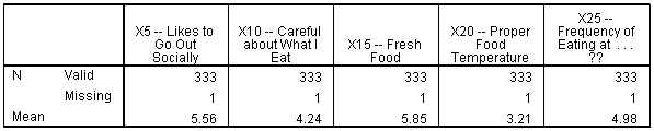
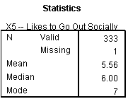
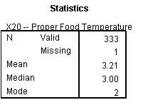
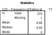
Mean value for X5 is 5.56, which shows that on an average, the respondents somewhat agree that they like to go out socially. Mean value for X10 is 4.24, which shows that on an average, the respondents are towards the neutral side about being careful of what they eat generally. Respondents agree, on an average, that they prefer fresh food. Maintaining a proper Food Temperature has been somewhat disagreed by respondents. Most of the respondents eat at restaurants very frequently.
One-Way Tabulation – Frequency Table
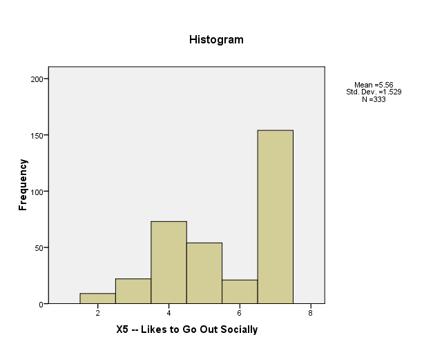
X5: Frequency table of “X5 – Likes to Go Out Socially” shows that most of the respondents strongly agree about their likeability to go out socially.

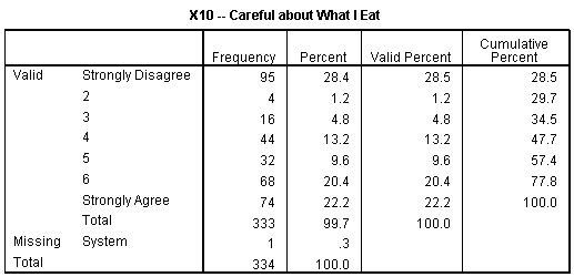
X10: The below given Frequency Table suggests that the respondents are more skewed towards either extremes, and consequently, they have remained almost neutral on an average.

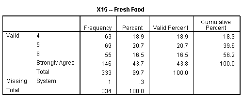
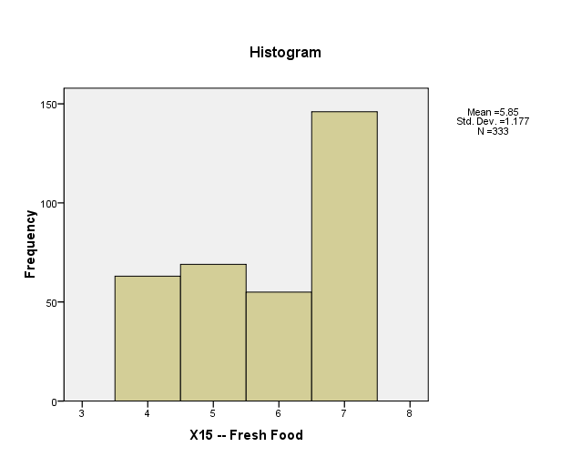
X15: Most of the respondents agree that Fresh Food is important for an individual, which is why their average mean score is inclined towards the Agree side.
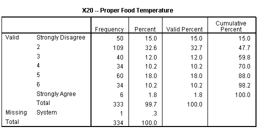
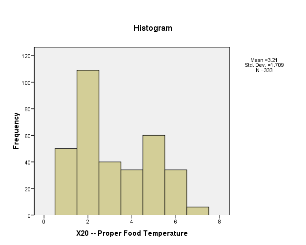
X20: A major portion of respondents disagrees with the importance of proper food temperature in a restaurant.
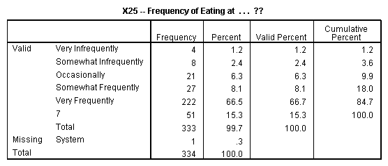
X25: Most of the respondents visit restaurants very frequently.

Mean, Median and Mode – Measures of Central Tendency
On an average, respondents somewhat agree towards their likeability to go out socially. However, the median score for X5 is 6.
On an average, respondents are unclear about careful consumption of food, while the median value revolves around “Somewhat Agree” opinion.

For the frequency distribution for Fresh Food importance and liking, the graph is skewed towards Agree side.

For the frequency distribution for importance of proper food temperature, the curve is skewed towards somewhat disagree side.
Most of the respondents prefer to eat in restaurants very frequently. This can be seen from the Statistics table providing Mean, Median, and Mode.
Range, Standard Deviation and Variance
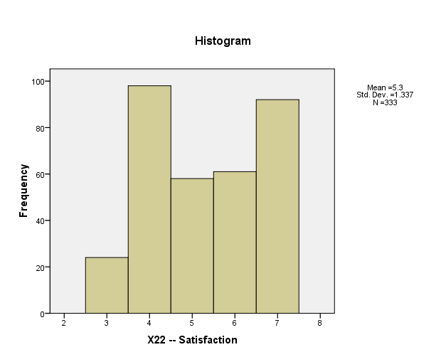
The variable X22 – “Satisfaction” has been taken into consideration here. The standard deviation of the responses is 1.337 with minimum value being 3 and maximum being 7. Respondents are more inclined towards agreeing on the satisfaction level.
|
Statistics |
||
| X22 — Satisfaction | ||
| N | Valid |
333 |
| Missing |
1 |
|
| Std. Deviation |
1.337 |
|
| Variance |
1.788 |
|
| Range |
4 |
|
| Minimum |
3 |
|
| Maximum |
7 |
|
Crosstabulation
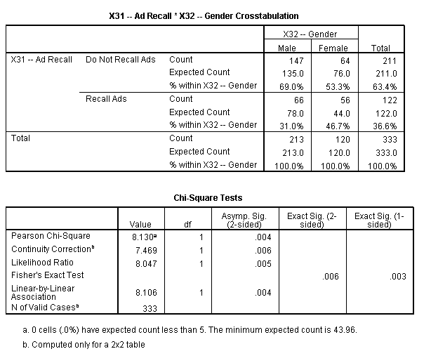
From the below output of Ad Recall and Gender crosstabulation table, it is evident that males tend to forget ads, while female are more capable of recalling ads.
|
X31 — Ad Recall * X32 — Gender Crosstabulation |
||||
| Count | ||||
|
X32 — Gender |
Total |
|||
|
Male |
Female |
|||
| X31 — Ad Recall | Do Not Recall Ads |
147 |
64 |
211 |
| Recall Ads |
66 |
56 |
122 |
|
| Total |
213 |
120 |
333 |
|
Crosstabulation – Testing for Differences with Chi-Square
Chi square test was done for testing the differences. The significance value for Chi square test is 0.006, which tells us to reject the null hypothesis. The null hypothesis in this case will be that “There is no impact of gender on ad recalling ability”. The Pearson Chi Square value is 8.130 and the Crosstabulation table also backs the rejection of null hypothesis as around 47% females are able to recall ads, whereas only 31% males are able to recall ads.
Compare Means of Two Groups
We performed a hypothesis testing with our Null hypothesis as there is no impact of gender on the likelihood of individual to recommend the restaurant.
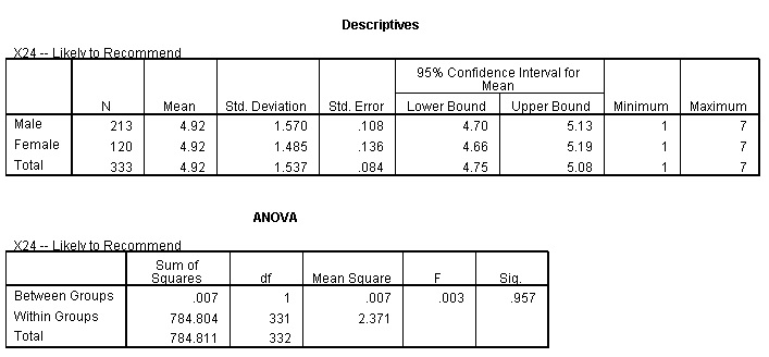
In the above ANOVA table, we can see that the Significance value is 0.957 and F value is 0.003. So, we fail to reject the null hypothesis. Thus, we can say that there is no impact of gender on the likelihood of recommending the restaurant.
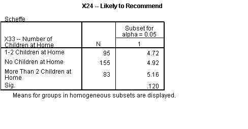
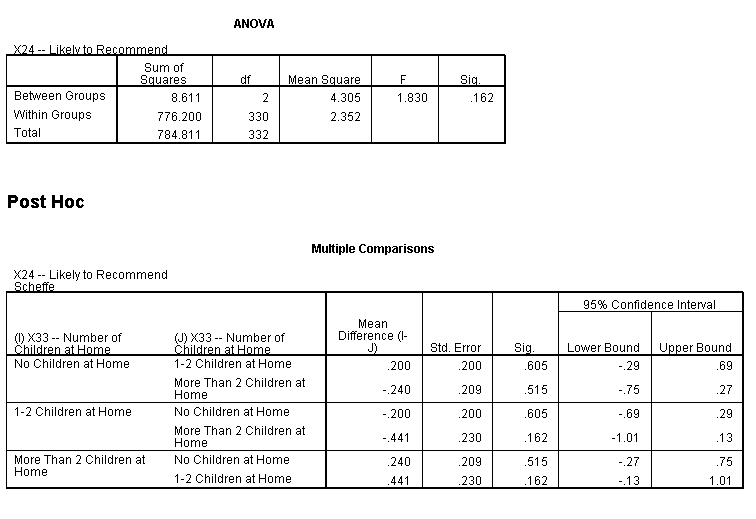
Compare Means of Three of More Groups
For this test, we take the No of children as one variable and tested if their likelihood of recommending is impacted by the no of children or not. Significance value is 0.162 and in the multiple comparisons table also, none of the p-values are significant. Hence, we fail to reject the null hypothesis and we can say that No of children and likelihood of recommending are not related to each other.
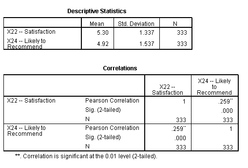
Pearson Correlation
The two variables taken into consideration are variable X22 (Satisfaction) and X24 (Likely to Recommend). We are trying to check if the satisfaction level affects the likelihood of recommending. Mean values for X22 and X24 are 5.3 and 4.92 respectively. Though the average score for X24 is lesser than X22, but the standard deviation is larger for X24 as compared to X22. The Pearson Correlation between these two variables is 0.259 at a significance level of 0.000. Hence, we will reject the null hypothesis that there is no correlation between satisfaction level and the likelihood of recommending. There exists a significant correlation.
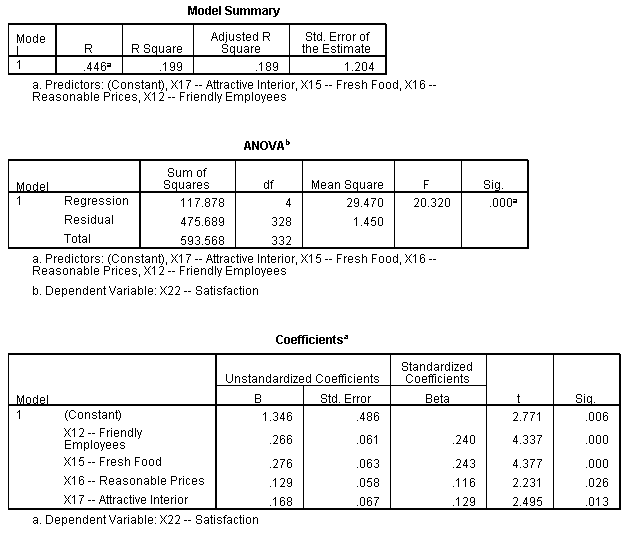
Multiple Regression
Here, we are trying to predict the satisfaction level based on 4 variables i.e. Friendly Employees, Fresh Food, Reasonable Prices, and Attractive Interior. From the below diagram, it can be seen that the regression model has 0.000 p value and F value as 20.230. The R2 square value for this model is 0.199, which is not great though. We can see that the significance value of all 4 variables is below the allowed limit of 0.05. Hence, we will not reject any variable, while formulating the regression model.
Final Model: –
Satisfaction = 1.346 + (0.266*Friendly Employees) + (0.276*Fresh Food) + (0.129*Reasonable Prices) + (0.168*Attractive Interior)
Looking for best SPSS Assignment help. Whatsapp us at +16469488918 or chat with our chat representative showing on lower right corner or order from here. You can also take help from our Live Assignment helper for any exam or live assignment related assistance.