StatCrunch Solved Homework Solution Sample

QUESTION

 

Problem 1: Appropriateness of Inference

For the following scenarios, answer the questions for each part.  In each part, the underlined text is the name of the StatCrunch data set to be used for that part.  Please note, do not conduct inference in either of these parts; just answer each question.

 

1. GPA Versus Seating Location. A professor wanted to know whether there was a difference in students’ grade point averages (GPA) depending on whether they sit in the front half of the classroom versus the back half of the classroom.  In a previous semester, a random sample of students was selected from the front of a classroom and another random sample was selected from the back of a classroom and each student’s current GPA was recorded.  The data provided in StatCrunch represent the GPAs from each random sample.  At the 0.01 significance level, can the professor conclude from these data that the mean GPA for front sitters is different from than back sitters?

 

1. What is (are) the parameter(s) of interest? Choose one of the following symbols (m (the mean of one sample); m_D (the mean difference from a paired (dependent) samples); m₁ – m₂ (the mean difference of two independent samples) and describe the parameter in context of this question in one sentence.

 

1. Depending on your answer to part (i), construct one or two relative frequency histograms. Remember to properly title and label the graph(s).  Copy and paste the graph(s) into your document.

 

• Describe the shape of the histogram(s) in one sentence.

 

1. Depending on your answer to part (i), construct one or two boxplots and copy and paste these graphs into your document.

 

1. Does the boxplot (or do the boxplots) show any outliers? Answer this question in one sentence and identify any outliers if they are present.

 

1. Considering your answers to parts (iii) and (v), is inference appropriate in this case? Why or why not?  Defend your answer using the graphs in two to three sentences.

 

1. GMU Health Center Waiting Time. During the flu season, it is known that the waiting time at the GMU Health Center can be extreme.  A statistics student wanted to test her claim that the wait time was greater than 100 minutes.  She took a random sample of wait times during the flu season and recorded them in StatCrunch.

 

1. What is (are) the parameter(s) of interest? Choose one of the following symbols (m (the mean of one sample); m_D (the mean difference of two paired (dependent) samples); m₁ – m₂ (the mean difference of two independent samples) and describe the parameter in context of this question in one sentence.

 

1. Depending on your answer to part (i), construct one or two relative frequency histograms. Remember to properly title and label the graph(s).  Copy and paste the graph(s) into your document.

 

• Describe the shape of the histogram(s) in one sentence.

 

1. Depending on your answer to part (i), construct one or two boxplots and copy and paste these graphs into your document.

 

1. Does the boxplot (or do the boxplots) show any outliers? Answer this question in one sentence and identify any outliers if they are present.

 

1. Considering the answers provided in parts (iii) and (v), is inference appropriate in this case? Why or why not?  Defend your answer using the graphs in two to three sentences.

 

 

Problem 2: Pizza Prices in Different Cities (no data set in StatCrunch)

A food blogger is interested in comparing the price of pizzas available for purchase in New York City to those available in Washington, D.C.  To do so, they collected a random sample of 30 large cheese pizzas from each of the cities.  The New York pizzas had an average price of $12.83 with a standard deviation of $4.45.  The Washington, D.C. pizzas had an average price of $10.71 with a standard deviation of $3.74.  At the 0.01 significance level, can the blogger conclude that the mean price of a large cheese pizza in New York is higher than Washington, D.C.?  Assume all conditions for conducting inference are satisfied.

 

1. Conduct a full hypothesis test by following the steps below. Enter an answer for each of these steps in your document.
   1. Define the population parameter of interest in context of this question in one sentence.
   2. State the null and alternative hypotheses using correct notation.

• State the significance level for this problem.

1. Calculate the test statistic in StatCrunch using STAT à T Stats à 2 Sample à With Summary. Copy and paste the output table into your document.
2. Label the p-value seen in your output table produced in part (iv) using the proper probability notation (it begins with P(…)).
3. State whether you reject or do not reject the null hypothesis and your reason for your answer in one sentence.

• State your conclusion in context of the problem (i.e. interpret your results and/or answer the question being posed) in one or two complete sentences.

 

1. Imagine if the significance level for this problem was 0.05. State your decision and conclusion for the above hypothesis test when you compare your p-value found in part (v) with the significance level of 0.05.

 

Problem 3: Food Prices: Target versus Safeway.  Grocery prices of the same randomly selected items were collected and compared from Target and Safeway.  Imagine you were interested in conducting a hypothesis test to determine whether the mean prices were significantly different.  Note: to answer the questions below, subtract Target price – Safeway price (i.e. subtract Safeway price from Target price).

 

1. Define the population parameter of interest in context in one sentence.

 

1. Calculate the difference between prices by subtracting Target – Safeway. List the difference for each of the 24 pairs in your document.  To calculate your differences using StatCrunch, you may use Data à Compute à  Click Build.  In this screen, Click on Target first, then click the minus sign, then click Safeway.

 

1. Produce a box plot of these differences and include it in your document. Comment in one sentence if any outliers are present.

 

1. Obtain the mean of these differences and the standard deviation of these differences in StatCrunch. You may copy and paste the box that you obtain from StatCrunch or list the values.  Please round the mean and standard deviation to four decimal places in your answer.

 

1. Construct a 95% confidence interval using the above data. Please do this “by hand” using the formula and showing your work (please type your work).  Use your t-table (found in the last page of our formula packet) to obtain your t* critical value needed for the confidence interval.  Present this confidence as (lower limit, upper limit).

 

1. Use StatCrunch to obtain a 95% confidence interval for the above data by selecting:

Stat à T Stats à Paired. Enter Target for Sample 1 and Safeway for Sample 2. Copy and paste your output into your document.

 

1. Imagine you were using a hypothesis test to determine if a significant difference exists in mean price between the two stores (the hypotheses would be H₀: m_D = 0 vs H_a: m_D ≠ 0). What conclusion can be made in this case using only your confidence interval?  Provide an answer and a reason for your choice in one or two sentences.  Again, please only use your confidence interval to answer this question (i.e. do not run this hypothesis test).

 

1. Verify your answer in part (g) by running a two-sided hypothesis test using StatCrunch. Only provide the StatCrunch output box.  Write one sentence describing your findings.

Problem 4: Variables that may affect Grades

The data set contains a random sample of STAT 250 Final Exam Scores out of 80 points.  For each individual sampled, the time (in hours per week) that the student spent participating in a GMU club or sport and working for pay outside of GMU was recorded.  Values of 0 indicate the students either does not participate in a club or sport or does not work a job for pay.  The goal of this problem is to explore the two time variables and see how each affects their Final Exam Score.  The Final Exam Score variable is the response variable in this problem.

1. Investigate the relationship between the explanatory variable “Club or Sport Time” and response variable “Final Exam Score” by doing the following:
2. i) Make a properly titled and labeled scatterplot and copy and paste it in your solutions (use Graph à Scatter Plot in StatCrunch).
3. ii) Calculate the correlation coefficient (use Stat à Summary Stats à Correlation in StatCrunch). Provide this value in your document.

• iii) Interpret the scatterplot and correlation coefficient in terms of trend, strength, and shape (form) in one complete sentence.

1. Investigate the relationship between the explanatory variable “Paid Job Time” and response variable “Final Exam Score” by doing the following:
2. i) Make a properly titled and labeled scatterplot and copy and paste it in your solutions (use Graph à Scatter Plot in StatCrunch).
3. ii) Calculate the correlation coefficient (use Stat à Summary Stats à Correlation in StatCrunch). Provide this value in your document.

• iii) Interpret the scatterplot and correlation coefficient in terms of trend, strength, and shape (form) in one complete sentence.

1. Which variable do you believe has the most effect on the Final Exam Score? Compare the two above R² values to make your decision.
2. Using the variable with the highest R² value as the explanatory variable, run a Simple Linear Regression analysis in StatCrunch. Use Stat à Regression à Simple Linear.  Copy and paste only the StatCrunch results output (no tables).
3. Add the fitted line plot to your document. This graph appears on page 2 of your output.
4. Type the regression equation into your document.
5. Interpret the slope of the regression line (in context of this data set).
6. Is it meaningful to interpret the y-intercept? Why or why not?
7. State R² (r-squared) (i.e., the coefficient of determination) and explain what this value means in context of the data set.
8. Use the regression equation from part (d) to predict the Final Exam Score for an individual who works 30 hours a week. State your predicted value in a sentence that is in context of the data.  Note:  You can do this calculation “by hand” or using StatCrunch.
9. Is your prediction in part (h) an example of extrapolation? Why or why not?

 

ANSWER

 

Problem 1. Appropriateness of Inference

1. a) GPA versus Seating Location:

(i) The grade point averages (GPA) of the students and their seating location in the classroom are the parameters of interest in this study.

μ_f (Mean GPA for the front sitters) = 3.237

μ_b (Mean GPA for the back sitters) = 2.971

The mean GPA for the front sitters is considerably higher than the back sitters.

(ii)

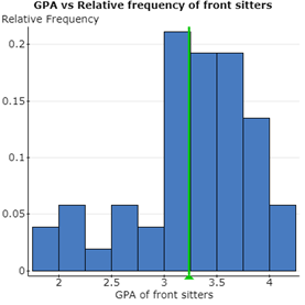
(iii) The relative frequency distribution for GPA of back sitters seems more right skewed, whereas the relative frequency distribution for GPA of front sitters seems to be left skewed one, with its mean being on the higher side than the former.

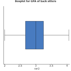
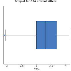
(v) The boxplot for GPA of front sitters shows an outlier, which is on the lesser extreme side. However, the boxplot for GPA of back sitters doesn’t show any outlier.

(vi) After looking at the above two graphs (relative frequency distribution and boxplot), we can infer that there is no statistically significant difference between the two means. There is an outlier for the front sitters GPA, and the range for relative frequency of GPA varies between front sitters and back sitters. However, at 5% significance level, there would have been a statistically significant difference.

 

(b) GMU Health Center Waiting Time

(i) Waiting time at the GMU Health Center during the flu season is our parameter of interest.

μ = 119.555 (The mean waiting time of the sample is 119.555 minutes at the GMU Health Center during the flu season.)

(ii)

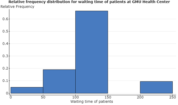
(iii) The shape of the histogram is left skewed near the mean but there is a gap in the later duration. There is a relatively very high frequency in the mean waiting time group.

(iv)

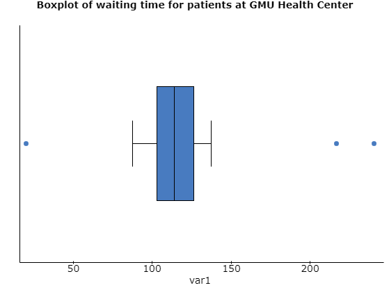
(v) The boxplot shows three outliers, two on the higher extreme and one on the lower extreme side. Apart from these three values, rest of the distribution looks similar to a normal distribution.

(vi) After looking at the above two graphs, the hypothesis testing in this case seems to be statistically significant, and for a 5% significance level, we can reject the null hypothesis that the mean waiting time for patients at GMU Health Center during the flu season is less than or equal to 100 minutes. The p-value would come to be lesser than 0.05.

 

Problem 2: Pizza Prices in Different Cities

(a) (i) The price of large cheese pizzas in USA is our population parameter, and we are comparing two samples from New York and Washington D.C. respectively.

(ii) H₀: There is no statistically significant difference between the mean price of large cheese pizzas in New York and Washington D.C.

H_A: The mean price of large cheese pizzas in New York is higher than that in Washington D.C.

(iii) The significance level for this problem is 0.01.

(iv

Two sample T summary hypothesis test:

μ₁ : Mean of Population 1
μ₂ : Mean of Population 2
μ₁ – μ₂ : Difference between two means
H₀ : μ₁ – μ₂ = 0
H_A : μ₁ – μ₂ > 0
(without pooled variances)

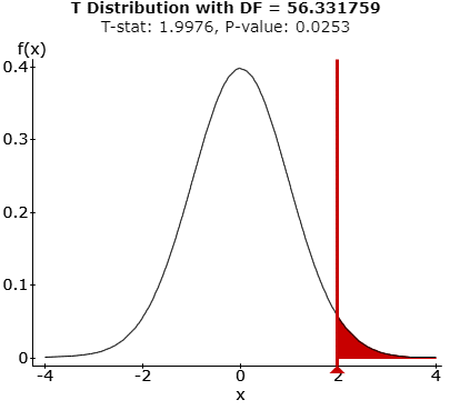
Hypothesis test results:

Difference	Sample Diff.	Std. Err.	DF	T-Stat	P-value
μ1 – μ2	2.12	1.0612901	56.331759	1.9975688	0.0253

 

(v) P-value comes out to be 0.0253.

(vi) As p-value is greater than the significance level at 0.01, we fail to reject the null hypothesis.

(vii) Thus, we can say that at 1% significance level, there is no statistically significant difference between the mean price of large cheese pizzas in New York and Washington D.C.

(b) If the significance level of the study is changed to 0.05, then the p-value of the hypothesis would be lesser than the accepted significance level, and hence, we would reject the null hypothesis. In other words, we can say that at 5% significance level, the mean price of large cheese pizzas in New York is higher than that in Washington D.C.

 

Problem 3: Food Prices: Target versus Safeway

(a) Prices of the food items from Target and Safeway are our population parameters in this study.

(b)

0
-0.2
-0.07
-0.3
1.4
-0.85
-0.76
-0.7
-0.96
-0.3
0.65
-2.25
-1.3
-0.1
-2
-0.2
0.19
-2.4
0.17
-0.07
-1.07
0.25
0
-1.3

 

(c) The boxplot is as below: –

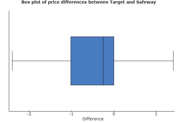
There is no outlier being shown in this boxplot. However, the above box plot is left skewed, as the positive price differences are closer than the negative price differences for the items.

(d)

Summary statistics:

 

Column	n	Mean	Variance	Std. dev.
Difference	24	-0.5071	0.8121	0.9012

(e) t-critical value for 23 degrees of freedom and 95% confidence interval = 2.0687

Std. dev = 0.9012

N=24

Mean = – 0.5071

Hence, the two limits would be as  – 0.5071 + {2.0687*0.9012/sqrt(24)} = – 0.5071 + 0.3806

The confidence interval is (- 0.8877, – 0.1265).

(f)

Paired T confidence interval:

μ_D = μ₁ – μ₂ : Mean of the difference between var2 and var3
95% confidence interval results:

Difference	Mean	Std. Err.	DF	L. Limit	U. Limit
var2 – var3	-0.50708333	0.18394675	23	-0.88760617	-0.1265605

(g) Both the upper and lower limits are having negative values i.e. values that are less than 0. Hence, if we run the hypothesis test in this case using only confidence interval, we can say that the test would be statistically significant, and we would reject the null hypothesis. Moreover, the standard deviation is having higher value in magnitude than mean, which has caused negative confidence limits.

(h)

Paired T hypothesis test:

μ_D = μ₁ – μ₂ : Mean of the difference between var2 and var3
H₀ : μ_D = 0
H_A : μ_D ≠ 0
Hypothesis test results:

Difference	Mean	Std. Err.	DF	T-Stat	P-value
var2 – var3	-0.50708333	0.18394675	23	-2.7566855	0.0112

We can say that we reject the null hypothesis and there is a statistically significant difference in the food prices of Target and Safeway.

 

Problem 4: Variables that may affect Grades

(a) (i)

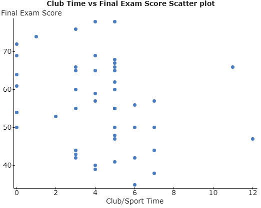
(ii) Correlation between var1 and var3 is: -0.24764239

(iii) We can see that most of the higher final exam scores are scored by those students, who spend lesser time for clubbing and sporting. Thus, we can see that the correlation is negative. Moreover, we can see that the points are dispersed throughout and not having much strength, which shows that the magnitude of correlation is lesser.

(b) (i)

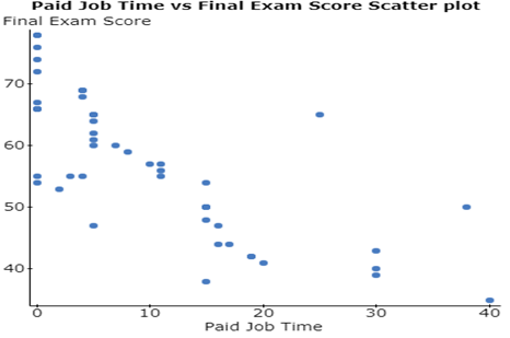
(ii) Correlation between var2 and var3 is: -0.74571401

(iii) We can see that the final exam scores have been higher for those students, who have been involved less in paid job time, which the correlation would be negative between the two variables. Moreover, the decrease in the scores with increase in paid job time seems to be more linear in this case, which is why the correlation magnitude would be higher.

(c) I believe that the paid job time has the most effect on the final exam score.

R² for the first correlation would be (– 0.2476)² = 0.0613

R² for the second correlation would be (– 0.7457)² = 0.5561

(d)

Simple linear regression results:

Dependent Variable: var3
Independent Variable: var2
var3 = 64.926009 – 0.80446118 var2
Sample size: 48
R (correlation coefficient) = -0.74571401
R-sq = 0.55608939
Estimate of error standard deviation: 7.6257517

Parameter estimates:

 

Parameter	Estimate	Std. Err.	Alternative	DF	T-Stat	P-value
Intercept	64.926009	1.5651442	≠ 0	46	41.482445	<0.0001
Slope	-0.80446118	0.10597456	≠ 0	46	-7.591078	<0.0001

 

Analysis of variance table for regression model:

 

Source	DF	SS	MS	F-stat	P-value
Model	1	3350.9831	3350.9831	57.624465	<0.0001
Error	46	2674.9961	58.152089
Total	47	6025.9792

(e)

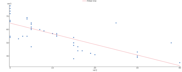
(f) Regression Equation:

Final Exam Score = [64.926 – 0.8045*(Paid Job Time)]

(g) The slope of this regression equation is – 0.8045, which shows the negative correlation between the paid job time and final exam score of a student.

(h) It is meaningful to interpret the y-intercept as it is putting a positive impact on the final exam score of the students.

(i) R² for this model comes out to be 0.5561, which tells us that the regression equation model explains around 55.6% of the variability of response data i.e. final exam scores around its mean.

(j) Final exam score for a student who works 30 hours a week = [64.926 – 0.8045*30] = 40.791

(k) Our prediction in part (h) is not an extrapolation because y-intercept is equal to that value of y when x becomes 0, and we already have several data points where the students have 0 job paid time.