QUESTION
Question 1: Formatting and charts (COs 1, 2, & 3; 30 points)
Using the Documentation sheet:
-
Enter your name and today’s date on the Documentation sheet.
Using the ‘Quest 1 & 2’ worksheet:
-
Select the Q1&Q2 sheet, and adjust the widths of the columns as needed.
-
Center the title “Super Shoes, Inc. Sales by Product” across columns A-D, increase the font size to 14 and change the font color to blue.
-
Bold the column headings “Product”, “Unit Price”, “Quantity”, and “Total Sales”.
-
Add formulas to the Total Sales column to calculate the total sales for each product.
-
Add a grand total at the bottom of the Total Sales column, in cell D8.
-
Format the numbers in the Unit Price and Total Sales columns as accounting or currency format with a dollar sign and two decimal places.
-
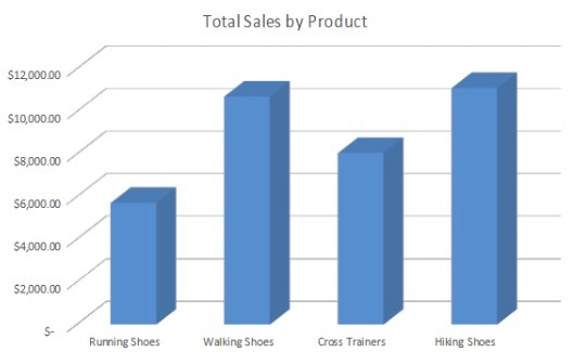
Create a 3-D column chart on a separate sheet that displays JUST the total sales for each product. (Do not include the grand total in the chart!)
-
Make the title of the chart “Total Sales by Product”.
-
Move the sheet with the column chart immediately after the Q1&Q2 sheet.
-
Rename the chart worksheet “Total Sales Chart”.
-
Save your work (CTRL+s) – (but leave it open to continue).
Question 2: Formulas, applications and Statistical Functions (COs 1, 4 & 9; 25 points)
Using the ‘Quest 1 & 2’ worksheet.
-
On the Q1&Q2 sheet, in cell E8, add a formula using a lookup function that will look up the grand total in cell D8 in the table of “Sales and Bonus” in A10:B13 and display the Bonus percentage. Use a range lookup. (For example, if the grand total in cell D8 was $15,500, then 5% should be displayed in cell E8.)
-
Format cell E8 as a percentage with zero decimal places.
-
In cell E10 enter the label Highest Sales. In F10 enter a formula using a function to display the highest total sales value for any product.
-
In cell E11 enter the label Lowest Sales. In F11 enter a formula using a function to display the lowest total sales value for any product.
-
In cell E12 enter the label Average Sales. In F12 enter a formula using a function to display the average total sales value for all products.
-
Format the labels and statistics (Highest Sales, Lowest Sales, and Average Sales) to display an outline (exterior border) around these cells for readability.
-
Add a brief comment to cell F10 to point to the highest in sales.
-
Save your work (CTRL+s) – (but leave it open to continue).
Question 3: Data cleansing, lists, sorting, conditional formatting, and pivot tables (COs 1, 4 & 8; 35 points)
Using the ‘Q3’ worksheet.
-
Adjust the widths of the columns so that the contents of each column are visible.
-
Add a new heading “Area Code” in cell I1. Column H contains each customer’s complete phone number. In column I, use the =MID() function to extract and display just the area code including the parentheses.
-
Convert the list of customers into an Excel table.
-
Sort the table into ascending alphabetical order by Last Name.
-
Apply conditional formatting to the State column so that cells containing “Texas” are highlighted in red and cells containing “California” are highlighted in yellow.
-
Convert the table back into a range.
-
Create a pivot table that uses State as the row field, no column field, and the count of Customer ID as the values.
-
Put your pivot table on a new sheet labeled Q3-Pivot and place this sheet immediately after the Q3 sheet.
- Save your work (CTRL+s) – (but leave it open to continue).
Question 4: Functions and Financials (COs 2, 6, and 7; 35 points)
Using the ‘Q4’ worksheet:
- Enter formulas in cells B4, B5, and B6 to calculate the total sales, total cost, and net income for a new product line, based on the projected unit sales, unit price, and unit cost provided.
- Adjust column widths as needed, and format all values except unit sales as currency with no decimal places.
- Assign the labels in column A as names for the corresponding cells in column B (that is, B1 should be assigned the name Unit_sales, B2 should be assigned the name Unit_price, and so on).
- Use the Scenario Manager to create three financial scenarios for this product: Most Likely, Best Case, and Worst Case.
- For the Most Likely scenario, unit sales are 50 units, unit price is $75, and unit cost is $45.
- For the Best Case scenario, unit sales are 100 units, unit price is $99, and unit cost is $40.
- For the Worst Case scenario, unit sales are 30 units, unit price is $60, and unit cost is $50.
- For all scenarios, results to calculate are Total sales, Total cost, and Net income.
- Create a Scenario Summary report sheet showing results for all three scenarios. Name the sheet ‘Scenario Summary’. Place the ‘Scenario Summary’ sheet immediately after the Q4 sheet.
LOAN ANALYSIS
- Super Shoes wants to apply for a 15-year loan and they need to know how much the monthly payment will be with a $15,000 down payment or a $30,000 down payment on a loan of $175,000. The annual interest rate is 3% and payment is assumed to be made at the end of the period.
- Complete the chart and calculate the monthly payment, using an Excel function.
- Secure/Protect, without a password, the Quest 4-Financials worksheet tab.
- Save your work (CTRL+s).
Question 5: Data consolidation and Analysis (COs 5, 3, 7, &8; 35 points)
Using the ‘Q5’ worksheets:
- Group the four sheets Q5 New York, Q5 Chicago, Q5 Los Angeles, and Q5 Summary. While the sheets are grouped, bold the labels in row 1 and column A, and format the values in cells B2:E5 as currency with no decimal places.
- While sheets are grouped add Totals to summarize quarters and products for each region and all regions.
- Ungroup the worksheets. Select the Q5 – Summary worksheet and use either data consolidate or 3D formulas to summarize the three locations into a total company.
- The summary sheet should display the totals for each product and quarter over all 3 cities (New York, Chicago, and Los Angeles).
- Format the Q5 – Summary totals with a single top and double bottom border across row 6 to frame the totals.
- Create a clustered column chart that shows total sales of each product in each quarter. Each cluster should represent a quarter, and each individual column should represent sales of a product within that quarter. Place your chart on the Q6- Analysis sheet. Give the chart an appropriate title.
- Add a trend line to the chart to show how sales of cross trainers are changing over time.
Question 6: Analysis Summary and Recommendation (COs 8 & 9; 15 points)
- In the space provided on the Q6 Analysis sheet, write a brief (2 paragraph) analysis report to the manager of the Super Shoes business. In your report, explain your findings on the trend in sales of cross trainers, and any other patterns you observed in sales of the product categories.
- In another paragraph, recommend at least one specific action that Super Shoes should take regarding the cross trainers product line.
- Save your work (CTRL+s) – (but leave it open to continue).
Question 7: Documentation Sheet and Summary (All COs 1 and 9); 25 points)
- Complete the documentation sheet with the following information:
- Purpose of workbook
- Sheet titles and Descriptions
- Class Conclusion: Your final conclusion about completing this course and what you learned (1 paragraph).
- Format the Documentation Sheet so that all information is easily readable and styled.
ANSWER
Documentation
| BIS-155 Final Exam Practical Problems | |
| Super Shoes, Inc | |
| Name: | Julia Cooper |
| Date: | 3/3/2019 |
| Purpose of workbook | ||
| The workbook highlights the financials and sales position of Super Shoes, Inc. and highlights the trends in the product line over the year. It also recommends the possible course of action for the company for its product. |
| Class Conclusion | |||||
| In the class we learned about the basic uses of Excel and how it can support a company in analysing its financials. Excel provides some powerful functions for a company to manage its finance data and understand the trends in its operations. We also saw how we can properly manage and represent data so that it becomes easier for the consumers to understand the data and navigate through the worksheet. |
| Sheet titles | Descriptions |
| Q1&Q2 | Super Shoes, Inc. Sales by Product |
| Total Sales Chart | 3D Chart of total sales per product |
| Q3 | Customer Details |
| Q3-Pivot | Customers per state |
| Q4-Financials | Basic Income Statement and EMI analysis |
| Scenario Summary | Scenarios for possible income statements |
| Q5 New York | Sales details per quarter per product for New York |
| Q5 Chicago | Sales details per quarter per product for Chicago |
| Q5 Los Angeles | Sales details per quarter per product for Los Angeles |
| Q5 Summary | Sales details per quarter per product for the company |
| Q6 – Analysis | Findings around sales (majorly cross trainers) and recommendations |
Q1&Q2
| Super Shoes, Inc. Sales by Product | |||||
| Product | Unit Price | Quantity | Total Sales | ||
| Running Shoes | $99.99 | 57 | $5,699.43 | ||
| Walking Shoes | $89.99 | 119 | $10,708.81 | ||
| Cross Trainers | $69.99 | 115 | $8,048.85 | ||
| Hiking Shoes | $74.99 | 148 | $11,098.52 | ||
| $35,555.61 | 10% | ||||
| Sales | Bonus | Highest Sales | The Highest sales are in Hiking Shoes $11,098.52 | ||
| 0 | None | Lowest Sales | $5,699.43 | ||
| 15000 | 5% | Average Sales | $8,888.90 | ||
| 30000 | 10% | ||||
Total sales chart
Q3
| Customer ID | Last Name | First Name | Street Address | City | State | Postal Code | Phone Number | Area Code |
| 3 | Adams | Martha | 7612 Sommers Crossing | El Paso | Texas | 88558 | (514)075-8644 | (514) |
| 1 | Butler | Daniel | 7513 Main Avenue | Albany | New York | 12242 | (336)572-1779 | (336) |
| 8 | Cook | Larry | 53 6th Parkway | Memphis | Tennessee | 38126 | (104)748-9720 | (104) |
| 12 | Cook | Charles | 88754 Brickson Park Court | Des Moines | Iowa | 50335 | (142)690-9166 | (142) |
| 17 | Fowler | Keith | 0472 Milwaukee Crossing | Fresno | California | 93709 | (893)437-0022 | (893) |
| 15 | George | Diane | 7096 Bayside Road | Boynton Beach | Florida | 33436 | (760)556-7300 | (760) |
| 10 | Greene | Eric | 80281 Golf View Circle | Biloxi | Mississippi | 39534 | (148)654-0304 | (148) |
| 6 | Hawkins | Andrew | 648 Arkansas Avenue | New Orleans | Louisiana | 70124 | (474)032-3827 | (474) |
| 14 | Howard | Dennis | 8352 Dennis Plaza | Des Moines | Iowa | 50330 | (985)899-2445 | (985) |
| 4 | King | Dorothy | 08799 West Alley | Tuscaloosa | Alabama | 35405 | (352)656-9412 | (352) |
| 7 | Moreno | Andrea | 12 Onsgard Way | Tucson | Arizona | 85725 | (862)349-3426 | (862) |
| 13 | Parker | Kenneth | 223 Waubesa Avenue | Norwalk | Connecticut | 6859 | (301)000-8630 | (301) |
| 18 | Parker | Bobby | 4661 Chive Street | New York City | New York | 10004 | (991)141-0734 | (991) |
| 20 | Rogers | Dorothy | 467 Shopko Point | San Diego | California | 92170 | (259)398-9977 | (259) |
| 19 | Romero | Mark | 52 Hagan Center | Erie | Pennsylvania | 16505 | (477)496-9649 | (477) |
| 9 | Ross | Kenneth | 60366 Kennedy Plaza | Lafayette | Louisiana | 70593 | (962)670-8039 | (962) |
| 5 | Wagner | Sharon | 53228 Killdeer Trail | Minneapolis | Minnesota | 55407 | (425)436-3366 | (425) |
| 16 | Walker | Carlos | 20 Boyd Crossing | Washington | District of Columbia | 20046 | (876)618-8692 | (876) |
| 11 | Weaver | Phillip | 29 Green Ridge Junction | Lexington | Kentucky | 40510 | (432)393-4362 | (432) |
| 2 | Williamson | Lois | 3 Artisan Trail | Houston | Texas | 77218 | (074)235-1480 | (074) |
Q3-Pivot
| State | Count of Customer ID |
| Alabama | 1 |
| Arizona | 1 |
| California | 2 |
| Connecticut | 1 |
| District of Columbia | 1 |
| Florida | 1 |
| Iowa | 2 |
| Kentucky | 1 |
| Louisiana | 2 |
| Minnesota | 1 |
| Mississippi | 1 |
| New York | 2 |
| Pennsylvania | 1 |
| Tennessee | 1 |
| Texas | 2 |
| Total Result | 20 |
Q4 Financial
| Net Income Chart | |
| Unit sales (quantity) | 50 |
| Unit sales price | $75 |
| Unit cost | $45 |
| Total sales | $3,750 |
| Total cost | $2,250 |
| Net income | $1,500 |
| Payment Function and Analysis (Part F & G) | |||||
| Down Payment | Present Value | Interest/Period | Loan Amount | # Periods | Payment |
| 15,000 | 175,000 | 0.0025 | 160,000 | 180 | $1,104.93 |
| 30,000 | 175,000 | 0.0025 | 145,000 | 180 | $1,001.34 |
| Scenario Summary | |||||
| Current Values: | Most Likely | Best Case | Worst Case | ||
| Changing Cells: | |||||
| $B$2 | 50 | 50 | 100 | 30 | |
| $B$3 | $75 | $75 | $99 | $60 | |
| $B$4 | $45 | $45 | $40 | $50 | |
| Result Cells: | |||||
| $B$5 | $3,750 | $3,750 | $9,900 | $1,800 | |
| $B$6 | $2,250 | $2,250 | $4,000 | $1,500 | |
| $B$7 | $1,500 | $1,500 | $5,900 | $300 | |
| Notes: Current Values column represents values of changing cells at | |||||
| time Scenario Summary Report was created. Changing cells for each | |||||
| scenario are highlighted in gray. |
| 1st Quarter | 2nd Quarter | 3rd Quarter | 4th Quarter | ||
| Running Shoes | $1,015 | $3,672 | $2,544 | $4,229 | $11,460 |
| Walking Shoes | $4,182 | $3,326 | $2,231 | $3,045 | $12,784 |
| Cross Trainers | $4,560 | $3,259 | $4,370 | $2,225 | $14,414 |
| Hiking Shoes | $2,562 | $3,862 | $4,512 | $3,669 | $14,605 |
| $12,319 | $14,119 | $13,657 | $13,168 |
| 1st Quarter | 2nd Quarter | 3rd Quarter | 4th Quarter | ||
| Running Shoes | $3,884 | $1,188 | $3,994 | $4,219 | $13,285 |
| Walking Shoes | $4,507 | $4,558 | $2,074 | $4,226 | $15,365 |
| Cross Trainers | $4,393 | $3,633 | $1,150 | $2,293 | $11,469 |
| Hiking Shoes | $3,466 | $2,851 | $2,023 | $3,338 | $11,678 |
| $16,250 | $12,230 | $9,241 | $14,076 | ||
| 1st Quarter | 2nd Quarter | 3rd Quarter | 4th Quarter | ||
| Running Shoes | $3,781 | $2,593 | $1,976 | $2,137 | $10,487 |
| Walking Shoes | $2,647 | $4,233 | $3,981 | $2,939 | $13,800 |
| Cross Trainers | $3,408 | $2,410 | $4,301 | $2,471 | $12,590 |
| Hiking Shoes | $2,333 | $1,285 | $3,751 | $2,523 | $9,892 |
| $12,169 | $10,521 | $14,009 | $10,070 | ||
| 1st Quarter | 2nd Quarter | 3rd Quarter | 4th Quarter | ||
| Running Shoes | #NAME? | #NAME? | #NAME? | #NAME? | #NAME? |
| Walking Shoes | #NAME? | #NAME? | #NAME? | #NAME? | #NAME? |
| Cross Trainers | #NAME? | #NAME? | #NAME? | #NAME? | #NAME? |
| Hiking Shoes | #NAME? | #NAME? | #NAME? | #NAME? | #NAME? |
| #NAME? | #NAME? | #NAME? | #NAME? | ||
| Analysis and Recommendation | |||||||||
| The total sales of the company for the year have been $151,829 out of which $38,473 have come of cross trainers. However we have seen a decline in the net sales of the product over the four quarters with the specially low sales in the 4th quarter. We have seen the same trend in all the three locations where the company operates, whereas on the other hand, product like the running shoes have seen a rise in the locations. Chicago is an exceptionally poor area where cross trainers are the worst performing products. They were the least selling products in chicago in two out of 4 quarters. When analysed with the data for all the locations this was the situation only for the last quarter for cross trainers. Having said that cross trainers are still the second most selling products and the company needs to increase the marketing expenditure on the product to sell more and make sure that the product does not see a continuous decline in sales for the next year as well. Conpany can also consider removing the product line from Chicago due to their poor performance in that market. |
|||||||||
Looking for best Accounting Assignment Help. Whatsapp us at +16469488918 or chat with our chat representative showing on lower right corner or order from here. You can also take help from our Live Assignment helper for any exam or live assignment related assistance